Jinli Liu, Wei Yu, Luoliang Xu, Xinjun Chen,＊, Wenjiang Guan, Gang Li

aCollege of Marine Sciences of Shanghai Ocean University, Shanghai, 201306, China

bLibrary of Shanghai Ocean University, Shanghai, 201306, China

cNational Distant-water fisheries Engineering Research Center, Shanghai Ocean University, Shanghai, 201306, China

dThe Key Laboratory of Sustainable Exploitation of Oceanic fisheries Resources, Ministry of Education, Shanghai Ocean University, Shanghai, 201306, China

ABSTRACT

Keywords:

Ommastrephes bartramii

Bayesian model

Bio-economic model

Management strategy

The northwest pacific ocean

1.Introduction

The neon flying squid (Ommastrephes bartramii) is widely distributed across the temperate and subtropical waters of the Pacific, Indian, and Atlantic Oceans (Ichii, Mahapatra, Okamura, & Okada, 2006). In the Northwest Pacific Ocean, the neon flying squid is one of the most important commercially targeted species for the distant-water fishing fleets of Chinese Mainland, Chinese Taiwan Province and Japan. This squid species has been commercially exploited by international squid jigging vessels (Wang & Chen, 2005). In 1993, Chinese Mainland started an exploratory fishery to investigate the resource and fishing ground of O. bartramii, and soon expanded the spatial scale of fishing ground. The main fishing ground was within the area of 38-46N and the west of 165E. Annual catch of O. bartramii caught by Chinese squid jigging vessels ranged from 80 × 10t to 100 × 10t (Chen, Qian, Liu, & Tian,2008). Since 1993, due to the large-scale high seas driftnet fishing was prohibited, Japanese squid jigging fishery mainly exploited O. bartramii by large-scale professional squid jigging vessels, and the annual catch was about 30 ×10t, but it significantly decreased after 2000. Chinese Taiwan Province mainly exploited O. bartramii through the bycatch of saury fishery fishing fleets, the annual catch was about 20 ×10t before 2000, then the annual catch was only one thousand tones after 2000(Wang & Chen, 2005).

Many studies have conducted analyses on the biology and fisheries of O. bartramii in the Northwest Pacific Ocean over decades, including the population structures, age and growth, migrations, formation and variation of fishing grounds, and fishing gravity centers and abundance forecasting ((Yatsu & Mori, 2000); Watanabe et al., 2004; Fan, 2004;Chen & Tian, 2006; Fan et al., 2010; Ma et al., 2011; Li, Chen, Liu, & Lu,2011; Tang, Wu, & Fan, 2011; Xu, Chen, & Yang, 2013; Yang, Chen,Feng, & Guan, 2013; Chen, Gong, Tian, Gao, & Li, 2013). At the same time, there have been some studies focused on stock assessment of O. bartramii. For example, based on large-scale squid driftnet data in Japan, Ichii et al. (2006) assessed the stock of the autumn cohort of O. Bartramii in the Northwest Pacific Ocean by the swept area method,DeLury method and the non-equilibrium surplus-production method. In addition, Chen et al. (2008a ,b, 2011) used the DeLury depletion method and a Bayesian Schaefer model to carry out the stock assessment and risk analysis of alternative management strategies for the winter cohort of O. bartramii. Cao, Chen, Tian, and Liu (2010) estimated the initial stock size of the western winter-spring stock of O. bartramii and its fishery management reference points. However, limited effort has been put into the area of bio-economic modelling and the economic evaluation of management strategies. fisheries resource exploitation is an integrated system involving factors such as resources biomass, biological characteristics, fishing methods, economic costs and so on, all which should be considered as a whole.

In this study, based on Schaefer surplus production model, a Bayesian Bio-economic model was established by using fishery data and relevant fishing economic data from the squid fishery in Chinese Mainland, Japan and Chinese Taipei during the period 1995-2008 in the Northwest Pacific Ocean. We assumed that the prior distributions for parameters follow uniform, normal and logarithmic normal in three different scenarios. We also calculated bio-economic reference points and evaluated different management strategies based on particular metrics. The results from this study could inform the squid fishery management.

2.Materials and methods

2.1.Data collection

The fisheries data of O. bartramii were obtained from the squid jigging fishery in the Northwest Pacific Ocean from 1995 to 2008 for this study. The fisheries data of Chinese Mainland were provided by Chinese Squid-jigging Technology Group in Shanghai Ocean University. The data included fishing dates (month and day), catch (unit: t), fishing efforts and fishing area (0.5×0.5as a fishing zone). The fishing ground was bounded between 38-46N and 150-165E. Catch per unit effort(CPUE) data was expressed in daily catch of a fishing vessel (unit: t/d·vessel). The fisheries data of Chinese Taiwan Province were collected from Taiwanese Overseas fisheries Development Council (http://www.ofdc.org.tw/index.htm). The fisheries data of Japanese squid-jigging vessels were collected from the Japanese fisheries Research Agency(http://kokushi.job.affrc.go.jp/index.html). The CPUE data in this study was standardized by Generalized Linear Bayesian Model (GLBM) (Cao et al., 2011; Lu, Chen, Cao, et al., 2013a, b). The annual standardized CPUE was considered as the relative abundance index of O. bartramii resources in the Northwest Pacific Ocean (Table 1). The economic data of O. bartramii such as cost and price were collected from Ningtai Oceanic fishery Co., Ltd. Zhoushan city, Zhejiang province. In recent years, single squid-jigging vessel operation cost was about 6000 RMB per day, and the average price was about 10 000 RMB per ton in the past five years.

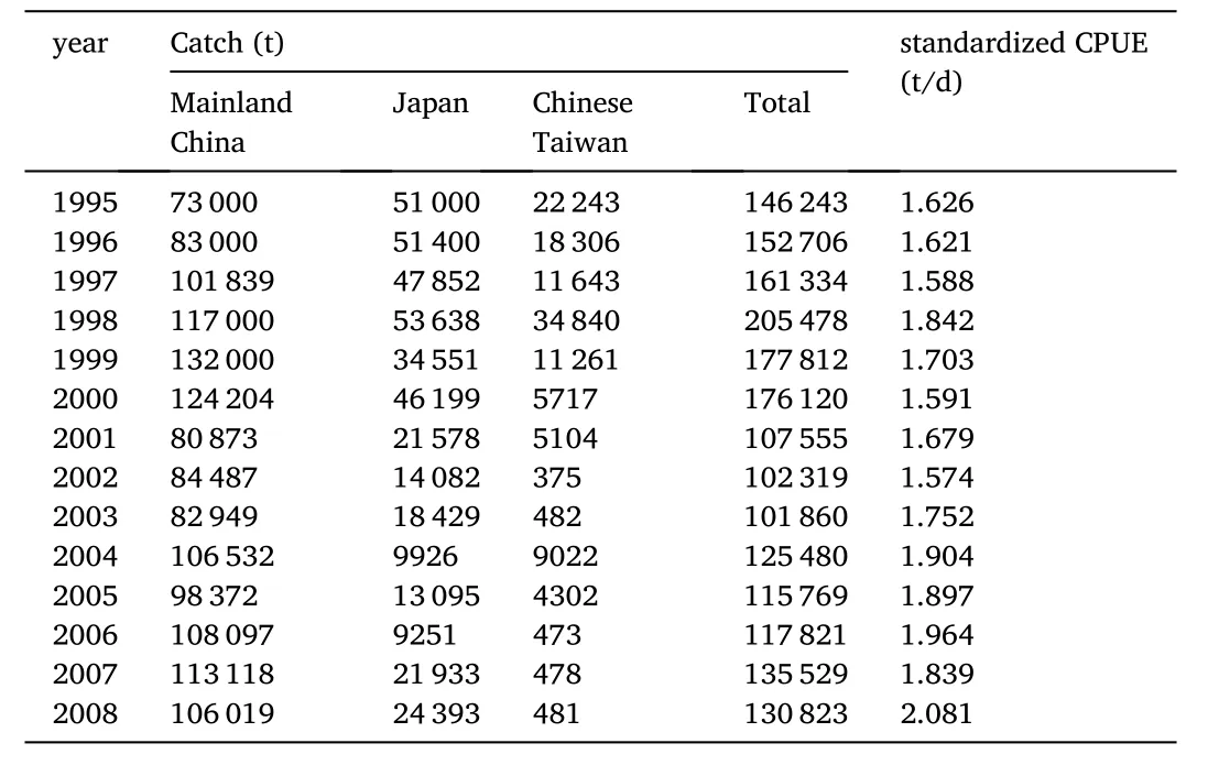
Table 1Catch and standardized CPUE data of O. bartramii for squid jigging fishery in the Northwest Pacific Ocean.

2.2.Schaefer surplus production model

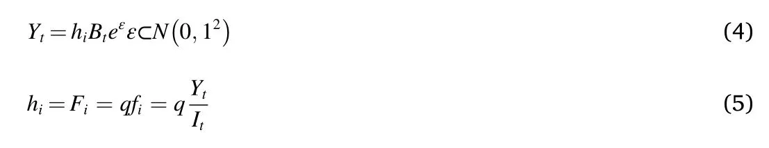
Schaefer resource dynamic model (Non-equilibrium surplus production model) was one of the most common models which were used in fishery resources assessment (Hilborn & Walters, 2001; Li, Chen, &Guan, 2010). The equations of this model can be expressed as:

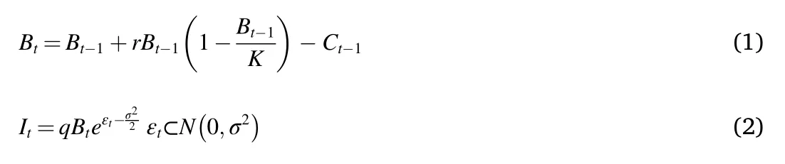
where Bwas the biomass at the year t; r was the intrinsic rate of growth;K was the carrying capacity, which was the equilibrium biomass before the fishery was exploited; Ywas the catch at year t-1; q was the catchability coefficient; Iwas CPUE at year t, and we assumed that Iwas proportional to B; εwas error term; σ was the standard deviation of CPUE.

In the actual stock assessment of fishery resource, we assumed that the biomass at the initial year when began to develop the fishery was equal to K (Mcallister & Kirkwood, 1998). Considering that Japan started O. bartramii fishery exploitation and utilization in 1973 in the Northwest Pacific Ocean, therefore, we could not consider the biomass of the first year in the time sequence as K in this study. We supposed that the initial biomass (B) of the O. bartramii in the Northwest Pacific Ocean as the biomass in 1995. According to the research results of Prager(1994) and Chen et al. (2011) and the fishery statistical data in Table 1,we inferred that the initial biomass (B) was about 400×10t.

2.3.Likelihood function

Actually, the likelihood function was a probability density function,which was used to estimate the goodness of fit between observation data and forecasting data of the model parameters(Li, Chen, & Guan, 2011).Assumed annual CPUE, namely Iwas directly proportional to B, and the observation errors were log-normally distributed, then the likelihood function equation was given as follows:

In this study, we analyzed fishery management strategies of the O. bartramii in the Northwest Pacific Ocean using the fishery data such as catch and CPUE data during 1995-2008, due to the time series of fishery data was short, the standard deviation (σ) was difficult to estimate, so we assumed it was equal to 0.2 (Mcallister & Kirkwood, 1998).

2.4.Setting prior distribution of model parameters

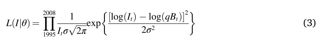
There were three scenarios (i.e., uniform distribution, normal distribution, and log-normal distribution) for the prior distribution of model parameters. These three scenarios represented the non-informative prior distribution, an informative prior distribution and lognormal effect of prior distribution (Table 2). Due to the significant in fluence of environmental variables on the stock of squid (Cao, Chen, &Chen, 2009), the model parameters r, K and q were also various.

According to the results of the stock assessment on O. bartramii in the North Pacific Ocean by Ichii et al. (2006), the intrinsic growth rate (r) of O. bartramii was set to 1.19. The baseline prior distribution for r was assumed following uniform distribution U (0.5, 2.0), normal prior distribution following normal distribution N (1.19, 0.6).

The baseline prior distribution for K followed uniform distribution U(500 × 10t, 1000 ×10t), the lower boundary was higher than the largest observed catch and initial biomass from 1995 to 2008, in order to reduce the in fluence of upper boundary on posterior probability,therefore, the upper bound was set at 100 thousand tons with normal prior distribution following normal distribution N (75, 37.5).

The prior distribution for q, the catchability coefficient, was set at 3.31 × 10-1.34 × 10, based on the findings from Cao (2010) and Liu, Chen, Li, and Wang (2014). Thus, we assumed the baseline prior distribution for q followed uniform distribution U(2.0 × 10-3 × 10), the prior distribution for q followed normal distribution N [2.5 × 10, (1.25 × 10)].

2.5.Estimating marginal posterior probability distribution

The Markov Chain Monte Carlo (MCMC) method was employed to estimate the posterior probability distributions for parameters r, K and q in the Schaefer surplus production model. The computing operation was achieved by R version 3.0.2 and Open Bugs 322. Initial values for r, K and q of the surplus production model in MCMC iterations were listed in Table 3. 50 000 runs were set, the results from the first 10 000 runs were discarded. Results from every 40 runs were stored.

Table 2Distribution scenarios and different settings for parameters r, K and q of prior distributions in the surplus production model.

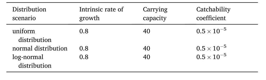
Table 3Initial value for r, K and q of surplus production model in MCMC iterations.

2.6.Determining the alternative management policy

The alternative management policies were set to different harvest rates (h) to examine changes in future catches and biomass. The harvest rate, also called fishing mortality rate (F), was a kind of harvest control rules (HCRs), which was used to understand the exploitation status of fishery resource, detect the equilibrium point between fishery resource and fishery industry. In this study, the harvest rates were set at 0, 0.1,0.2, 0.3, 0.4, 0.5, 0.6, 0.7 and 0.8, respectively. The catch in the future year t could be estimated by the following equations:

Where Ywas the catch in the year t in the management period; hwas the harvest rate; Bwas the biomass in the year t in the management period; ε was error term; fwas the fishing effort in the year t in the management period.

2.7.Gordon-Schaefer Bio-economic model

The general equations for Gordon-Schaefer Bio-economic Model were expressed as follows:

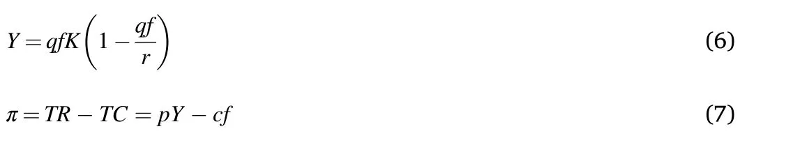
where π was the profit; TR was the total income; TC was the total cost; p was the price; Y was the catch; f was the fishing effort; c was the cost per fishing effort (Chen, 2004; Clark, 1985, 1990; Yagi, Ariji, Takahara, &Senda, 2009). Based on this model, we estimated the maximum sustainable yield (MSY), maximum economic yield (MEY), bio-economic balance point (BE), and the corresponding catch and economic incomes under different alternative management policies.

2.8.Evaluating the management reference points for fishery management

The management reference point could be divided into biological reference point (BRP) and economic reference point (ERP) (Caddy,1998; Jackson, 1994; Tong, Chen, Tian, Zhang, & Chen, 2010). The BRP in this study included F, B, Fand MSY. Fand Brespectively indicated the fishing mortality rate and biomass when the fishery reached the maximum sustainable yield. Findicated the fishing mortality rate where the slope of the YPR curve was 10% of the maximum slope, and now it is regarded as a more appropriate management target (Grabowski & Chen, 2004). The ERP consisted of MEY,F, B, BE, Fand B. Fand Brespectively indicated the fishing mortality rate and biomass, when the fishery reached the maximum economic yield. Fand Brespectively indicated the fishing mortality rate and biomass when the fishery reached the bio-economic balance point (Table 4).

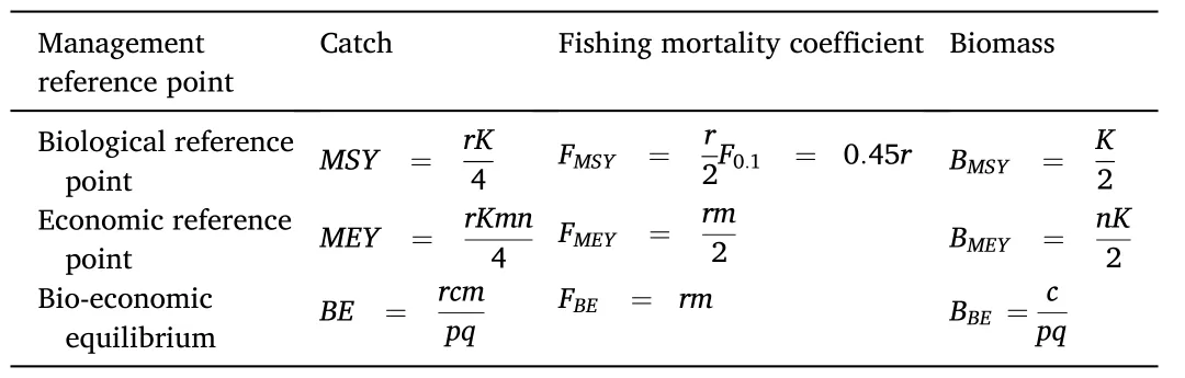
Table 4The fishery management reference points of O.bartramii in the Northwest Pacific Ocean.

In this study, Fwas considered as a target reference point of fishing mortality (F); Fwas considered as a limit reference point (F);Bwas considered as a target reference point of biomass (B); B/4 was considered as a limit reference point (B). The stock status (i.e.,over fishing or over fished) was determined by comparing the estimated fishing mortality and biomass in the terminal year with the limited reference points.

2.9.Evaluating management strategies and risk analysis

We used 10 metrics to evaluate the potential consequences of the alternative management strategies. The management time was from 2009 to 2023. The indices of policy performance were listed as follow:

(1) the biomass in 2023 (B);

(2) the catch in 2023 (Y);

(3) the minimum biomass (B) from 2009 to 2023;

(4) the expected value of the ratio of B/B;

(5) the depletion in 2023 (B/K);

(6) the probability that Bwould be larger than B(B＞B);

(7) the probability that the resource would be at a healthy level, i.e.,the probability that Bwould be larger than B(B＞B);

(8) the probability that the resource would be collapsed, i.e., the probability that Bwould be lower than B/4 (B＜B/4);

(9) the probability that Bwould be larger than B(B＞B);

(10) compare the cumulative catch and economic incomes in short term (2009-2013, 5 years), median term (2009-2018, 10 years),and long term (2009-2023, 15 years) by different management strategies;

We should balance the reservation (Band B) and exploitation(total catch, economic incomes and social benefits) of squid resource.The fishery management decision should base on the principle that the highest of expected revenue and the lowest risk of resource collapse in order to achieve the sustainable exploitation of squid resource (Chen et al., 2011).

3.Results

3.1.Posterior probability distributions for parameters r, k and q

Figs. 1-3 showed the MCMC sampling process and marginal posterior probability distribution for r,K and q under different distribution scenarios. Among the three scenarios, great difference was found between the marginal posterior probability distributions and the assumed prior probability distributions for parameters r and K, indicating that the fishery data strongly affected the marginal posterior probability distributions for parameters r and K. Under the normal scenario, the difference between the marginal posterior probability distributions and the assumed prior probability distribution for parameter r was the most obvious. It suggested that parameter r was not completely following normal distribution and had high uncertainty (Fig. 2). Small difference was found between the marginal posterior probability distributions and the prior probability distribution for parameter q, indicating that the posterior probability distribution for q basically followed normal distribution (P ＜0.05) and had low uncertainty.

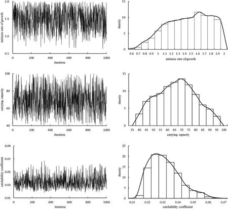
Fig. 1.MCMC sampling process (left) and density distributions (right) for r, K and q under uniform distribution scenario.

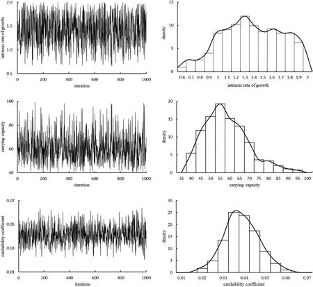
Fig. 2.MCMC sampling process (left) and density distributions (right) for r,K and q under normal distribution scenario.

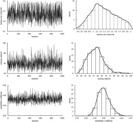
Fig. 3.MCMC sampling process (left) and density distributions (right) for r, K and q under log-normal distribution scenario.

Posterior means and standard deviation for model parameters for the three prior distribution scenarios were summarized in Table 5. Parameter r ranged from 1.346 to 1.489, with its lowest value occurring under the normal scenario and highest value occurring under the uniform scenario. Parameter K ranged from 59.84 × 10tons to 69.33 × 10tons,with its lowest value occurring under the lognormal scenario and highest value occurring under the uniform scenario. Parameter q ranged from 0.345 × 10to 0.425 × 10, with its lowest value occurring under the uniform scenario and highest value occurring under the lognormal scenario. Small difference was found for parameter q among the three scenarios, suggesting convergence in MCMC runs.

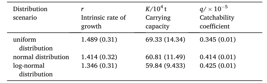
Table 5Posterior means and standard deviation for model parameters for the three prior distribution scenarios.

3.2.Current status of O. bartramii stock biomass

The biomass and the status of exploitation for O. bartramii during 1996-2008 in the Northwest Pacific Ocean in different distribution scenarios were shown in Fig. 4. The biomass of O. bartramii was much higher than the target reference point

B

and the bio-economic reference point

B

. The fishing mortality rate of

O. bartramii

fishery was much lower than the target reference point

F

and the bioeconomic reference point

F

. Therefore, our findings suggested that the stock was not over fished and over fishing did not occur. The stock status and the exploitation rate were at a healthy level in terms of economy.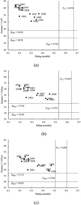

Fig. 4.Relationship between O. bartramii and management reference points from 1996 to 2008 under different distribution scenarios. (a) Uniform distribution; (b) normal distribution; (c) log-normal distribution.

The estimated fishery management reference points of

O. bartramii

were summarized in Tables 6-8 for the scenarios of the uniform distribution, normal distribution and lognormal distribution, respectively. In the uniform scenario, the estimated MSY was 25.55 ×10t and the corresponding

B

was 38.56 × 10t; the MEY and BE was 23.61 × 10t and 20.24 × 10tons, respectively, corresponding to 44.00 × 10t

B

and 18.67 ×10t

B

. The values in the normal and lognormal scenarios (Tables 7 and 8) were similar, but were obviously lower than those in the uniform scenario (Table 6). The estimated management reference point was the lowest in the lognormal scenario. In this scenario, the estimated MSY was 19.57 ×10t, corresponding to 29.92 × 10t

B

; the MEY and BE was 18.37 × 10t and 14.48 × 10t,respectively, corresponding to 37.13 × 10t

B

and 14.41 × 10t

B

.For the reference point

F

,

F

and

F

, small differences were found among different scenarios. The

F

,

F

and

F

in the uniform scenarios were respectively 0.670, 0.744 and 0.542, which were the highest among the three scenarios. The

F

,

F

and

F

were the lowest in the lognormal scenario, of which the values were 0.606, 0.673 and 0.506, respectively. The results from all scenarios supported the fact that the fishing mortality rate was much lower than

F

and

F

, and the current catch level was lower than the MSY.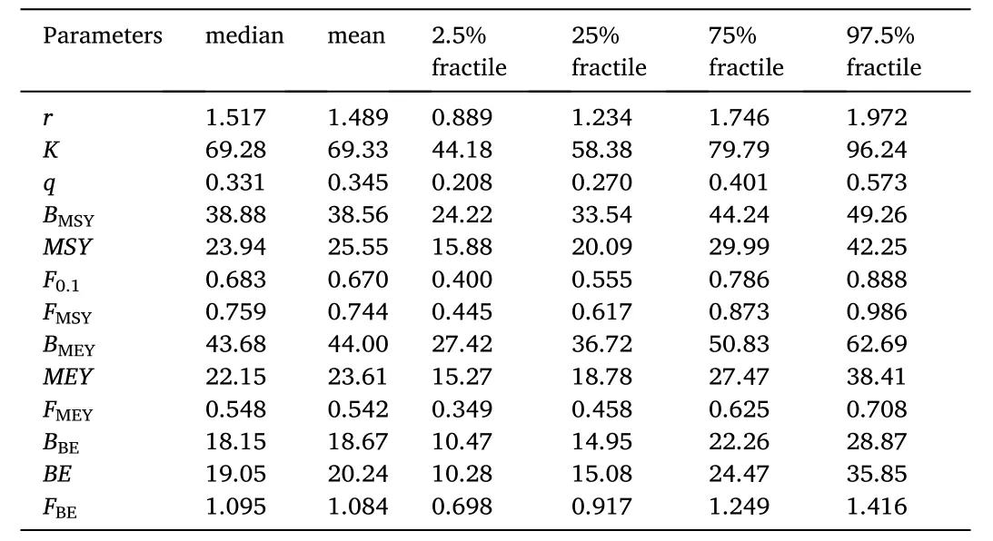

Table 6Summary statistics for the estimated fishery management reference points of O. bartramii for the uniform distribution scenario.

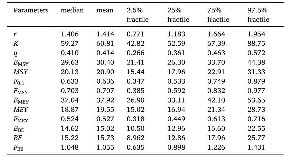
Table 7Summary statistics for the estimated fishery management reference points of O. bartramii for the normal distribution scenario.

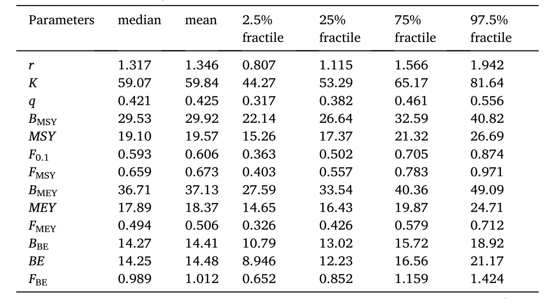
Table 8Summary statistics for the estimated fishery management reference points of O. bartramii for the log-normal distribution scenario.

3.3.Decision analysis and risk analysis

Comparing the indices in Table 9, small difference was found for the indices between normal and lognormal scenarios with different harvest rate, the values were lower than those in the uniform scenario. The estimated expected values of B, catch and the observed minimum biomass were higher than those in the other two scenarios. When the harvest rate was set to 0.7, the expected value of Ywas 24.28 ×10t and 19.61 ×10t, respectively, in the uniform and normal scenario,corresponding to 34.67 × 10t Band 27.99 × 10t B, respectively. With the harvest rate =0.6, the expected value of Ywas 18.46 × 10t under the lognormal case, corresponding to 30.76 × 10t B. However, the expected value of Ywas 23.75 ×10t and 19.55 ×10t, respectively, under the uniform and normal case, which were slightly lower than the expected values of maximum catch. The expected value of Bwere 39.58 × 10t Band 32.58 × 10t,respectively, under the uniform and normal case, which were higher than those when the harvest rate was equal to 0.7. From the analyses above, we could conclude that the harvest rate should be maintained at 0.6 for achieving the maximum yield during 2009-2023, the biomass of O. bartramii would range from 30.76 × 10t to 39.58 × 10t.

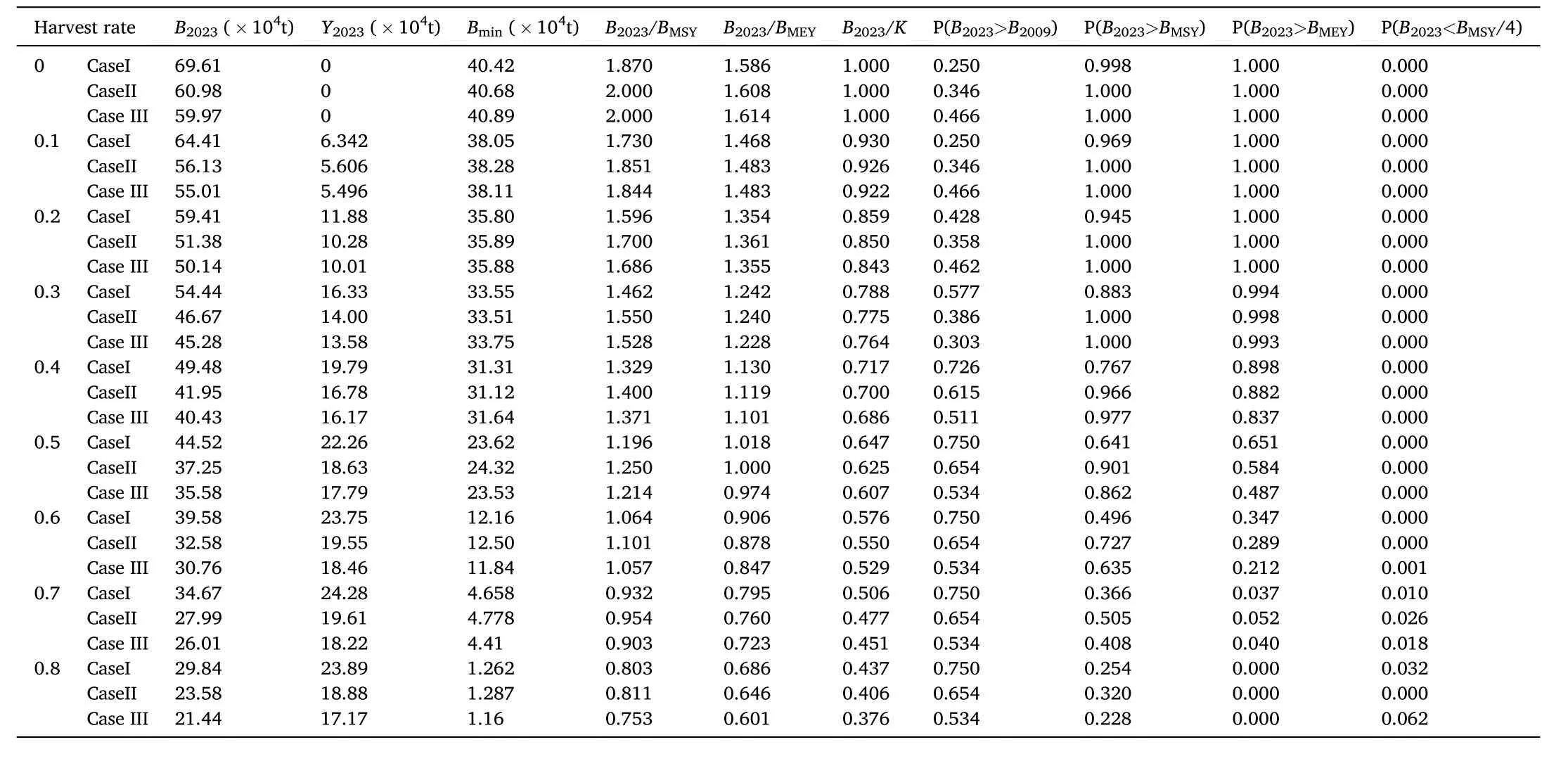
Table 9Summary statistics for the estimated index for management strategy and risk analysis of O. bartramii under the scenarios of uniform, normal and log-normal distribution.

However, if the harvest was set to 0.6, the results from all the three scenarios were pessimistic in terms of the estimated biomass in 2023.The minimum Bwas relatively high in the normal scenario with the value was only 12.50 ×10t. The estimated expected values of B/Bwere higher than 1 in all the three scenarios with highest value of 1.101 in the normal scenario. The expected values of B/Bwere 1.064 and 1.057, respectively, in the uniform and lognormal scenario,and were slightly lower than those under the normal scenario. For the P(B＞B) which indicated that the biomass was at the healthy level,difference was found among the three scenarios. P(B＞B) was 0.496, 0.727 and 0.635 in the uniform normal and lognormal scenario,respectively. For the P(B＜B/4) which indicated that the stock was collapsed, P (B＞B) was 0.00. For the P(B＞B), the value was only 0.212 in the lognormal scenario and was 0.347 in the uniform scenario. In conclusion, when the harvest rate was set to 0.6 in the uniform scenario, the expected value of Bwas slightly larger than the B, which would not result in the collapse of the stock.However, the probability of the expected value of Blarger than the Bwas less than 50%, suggesting the stock would decline. Therefore,if the squid stock was exploited by 0.6 harvest rate, the biomass would probably collapse. While in the normal and lognormal scenario with the harvest rate equal to 0.6, the expected value of Bwas much larger than the B, maintaining at a high level. Furthermore, the probability of the expected value of Blarger than the Bwas high, the probability that the stock collapsed was low. However, the biomass was over fishing at the economic aspect.

After the management measures were implemented, we analyzed the accumulative catches and profits of O. bartramii fishery in short, medium and long-term for the scenarios of uniform, normal and normal distribution (Fig. 5). Results suggested that in the normal scenario with the harvest rate equal to 0.6, the cumulative catchs in short, medium and long-term were the highest, corresponding to 94.53 ×10t,200.28 × 10t and 279.51 × 10t, respectively. When the harvest rate was 0.5, the cumulative catch was at intermediate level. However, the cumulative profits were highest, corresponding to 54.90 ×10RMB,114.71 × 10RMB and 162.34 × 10RMB in short, medium and longterm (Fig. 5-III). With respect to the uniform and normal scenario, thecumulative catch reached the highest value when the harvest rate was equal to 0.7. The cumulative catch in the uniform scenario were 119.21 × 10tons, 254.08 × 10t and 362.1 × 10t, respectively, in short, medium and long-term. For the normal scenario, the cumulative catch was 99.89 × 10t, 211.74 × 10tons and 296.76 × 10t, respectively, in short, medium and long-term. However, the cumulative profits reached the highest value when the harvest rate was equal to 0.6, The cumulative profit under the uniform case was 67.22 ×10RMB,139.52 × 10RMB and 202.96 × 10RMB, respectively, in short,medium and long-term. For the normal case, the cumulative catch was 57.70 × 10RMB, 120.58 × 10RMB and 171.64 × 10RMB, respectively, in short, medium and long-term (Fig. 5-Iand 5-II).

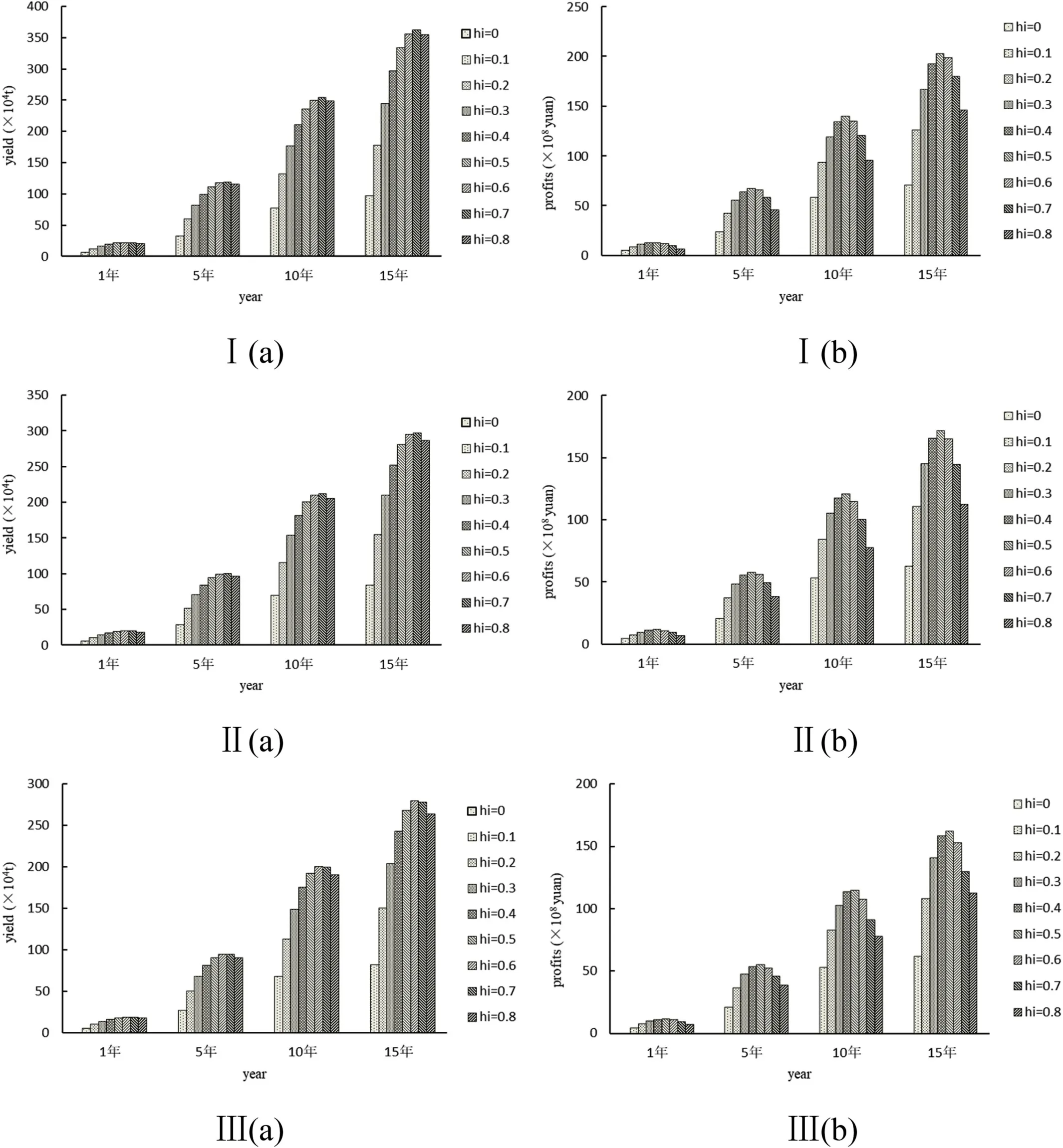
Fig. 5.The accumulative catches and profits of O. bartramii fishery in short, medium and long-term under the scenarios of uniform distribution, normal distribution and normal distribution. I: uniform distribution; II: normal distribution; III: log-normal distribution.

With the specific harvest rate, the catch and biomass were highest in the uniform scenario, however, the indices for the decision analysis was pessimistic. Regarding to the normal and lognormal scenario, the indices for the decision analysis showed similar trend. In the uniform scenario, it was suggested that the best management measure was to set the harvest rate equal to 0.4 for the O. bartramii fishery in the Northwest Pacific Ocean, the MSY was about 20 ×10t; In the normal and lognormal scenarios, the preferred management measure was to set the harvest rate equal to 0.5 for the O. bartramii fishery, the MSY was about 18 ×10t,which could maintain high catch and also high profits. The biomass could be stable and higher than the B.

4.Discussion

4.1.Prior and posterior distribution

Bayesian stock assessment methods provide useful information to obtain the posterior probability of parameters and reference points. How to select the prior distributions for parameters can greatly affect the posterior probability distribution. In recent studies, there was still many different opinions in selecting prior probability distribution (Walters &Ludwig, 1994). A potential error could exist in the results from the stock assessment due to the inappropriate prior information (Chen, Breen, &Andrew, 2000; Mcallister, Pikitch, & Babcock, 2001; Punt & Hilborn,2001). For example, if the data we used are non-informative, the prior probability distribution could greatly dominate the posterior probabilities (Punt & Hilborn, 2001; Stobberup & Erzini, 2006).

In this study, the prior distribution for model input parameters of r, K and q were set based on previous studies. We developed three scenarios of the prior distributions for model parameters (i.e., uniform distribution, normal distribution and lognormal distribution). Our results indicated that there was a small difference between the marginal posterior probability for q among the three scenarios and the assumed prior probability distribution. Additionally, the posterior probability for q basically followed the normal distribution, suggesting this parameter had low uncertainty in the Bio-economic model based on the Bayesian method. The results of the assessment might be insensitive to the prior distribution for q. For parameters r and K, the great difference was found between the marginal posterior probability for r and K under the three cases and the assumed prior probability distribution, which could introduce large uncertainty in the model. All these indicated that our data provide enough information about the values of the model parameters under each of the assumptions of their priors.

4.2.Analysis of the current status of O. bartramii stock biomass

Based on the statistical data from the squid fishery in China, Japan,and Chinese Taiwan Province during 1995-2008, the annual catch of O. bartramii ranged from 10 × 10t to 20 × 10t, the average catch was about 14 × 10t. The highest catch was 20.55 × 10t in 1998, followed by the second highest catch 17.78 ×10t in 1999. The estimated minimum MSY under the three cases was 19.57 ×10t. All the catches from 1995 to 2008 except in 1998 were lower than the minimum MSY. The fishing mortality rate of O. bartramii over 1996-2008 was lower than the F, suggesting that the squid stock was not over fishing. Furthermore,the annual biomass was higher than the B, indicating the biomass of O. bartramii was at a high level. Therefore, our result suggested the current statues of O. bartramii stock in the Northwest Pacific Ocean was optimistic, squid stocks was not over fishing in the recent decade years.Our findings were consistent with the results from Cao, Chen, Liu, and Tian (2010); Cao, Chen, Tian, and Liu (2010). The estimated MSY in this study was about 20 ×10t, which was different from previous studies.The difference might be caused by the different assessment model, the source of fishery data and different model parameters setting.

4.3.Analysis of management measures for O. bartramii

The selection of management measures by the fishery managers should follow the rule that achieves sustainable fishery with high catch and profits. Our results suggested the squid fishery could obtain the maximum sustainable catch and economic profits when the harvest rate was set to 0.6. However, in this situation, the probability that the Bis higher than Bwas very low, implying that the squid stock had the potential risk to collapse. Therefore, the harvest rate setting to be 0.4 should be the best measure in the uniform scenario, the MSY was about 20 ×10t; for the normal and lognormal scenario, the harvest rate should be set to 0.5, the MSY was about 18 ×10t. In summary, setting the harvest rate between 0.4 and 0.5 should be the best fishery management measures, in which the objective of sustainable high catch and profits could be achieved.

4.4.Uncertainty

The uncertainties in fishery management derived from different sources, such as the process error yielded by the random character of the dynamics of fishery resources, observation or measurement errors from collecting the fishery data and the uncertainty of model parameters(Chen & Paloheimo, 1998; Patterson, Cook, & Darby, 2001). The Bayesian theory was largely applied to fish stock assessment and management due to it ability to account for uncertainties related to models and parameter values. Due to the short life span of squid species, the stock biomass was strongly in fluenced by the climatic and environmental conditions (Chen, Liu, Tian, Qian, & Li, 2009; Rodhouse, 2001).Therefore, the absence of environmental variables in our model would introduce some risks in the evaluation of management measures.

Acknowledgements

We thank the Chinese distant-water Squid Jigging Technical Group for providing fishery data and information, and we thank NOAA for providing the environmental data used in this paper. This work was funded by Natural Science Foundation of China (41876141), the Funding Scheme for Training Young Teachers in Shanghai Colleges and the Shanghai Leading Academic Discipline Project ( fisheries Discipline).