YOU Yang, JIN Guang, PAN Zhengqiang, and GUO Rui

1.College of Systems Engineering, National University of Defense Technology, Changsha 410073, China;

2.Institute of Systems Engineering, Academy of Military Sciences, Beijing 102300, China

Abstract: Iterated local search (ILS) is used to construct the optimal experimental designs for multi-dimensional constrained spaces, in which the inner loop is based on the stochastic coordinate-exchange (SCE) algorithm.Every time a local optimal solution is found by the SCE algorithm, the perturbation operator is applied to it, and then a new solution is explored in the areas where the exchange of coordinates may produce improvement, so as to retain the features and attributes of the current optimal solution and avoid the defects of random restart.We implement the iterated local coordinate-exchange algorithm for experimental designs in the multi-dimensional constrained spaces.In addition, sensitivity analysis was conducted to analyze the impacts of the parameters on the performance of the proposed algorithm.Also we compared the performance of the proposed algorithm to the SCE algorithm using the random restart strategy.The analysis shows that the proposed algorithm is better than the SCE algorithm in terms of efficiency and quality, especially in the experimental designs for high-dimensional constrained space.

Keywords: constrained space, experimental design, coordinateexchange, iterated local search (ILS).

1.Introduction

Design of experiment (DOE) studies how to select design points from the design space according to the predetermined target, so as to explore the behavior of the response in the design space in the most economical and effective way [1].In many practical applications, constraints are imposed on the factors, resulting in multiple factors which are not independent and the design space which is not a regular hypercube.At present, the construction of experimental designs for constrained space mainly depends on the local search for candidate-set[2?6], which is difficult to be implemented in highly constrained space.In 1995, Meyer proposed the coordinateexchange algorithm [7], which is different from the traditional local search algorithms.Since it does not use candidate-set, the solution space to be explored is not restricted, and it is suitable for convex constraints, so it has been widely used in the field of experimental design[8?12].The main limitation of the coordinate-exchange algorithm is its tendency to fall into local optimum, especially when it is applied to experiments with a larger number of factors and observations.Kang provided a stochastic coordinate-exchange (SCE) algorithm [13] for constructing optimal experimental designs for linear, nonlinear, convex, non-convex and any irregular constrained space, which extends the scope of application of the coordinate-exchange algorithm.The SCE algorithm improves the design by exchanging coordinates stochastically, and overcomes the problem of easily getting trapped in locally optimal designs by executing the algorithm several times (that is, restarting the search with different initial designs).It is found that the restart strategy only expands the scope of search and increases the probability of getting trapped in locally optimal designs; in addition,the strategy lacks stability and is not suitable for largescale experimental designs [14,15].

Iterated local search (ILS) belongs to a category of multi-start metaheuristics that improves the performance of the simple random restart by incorporating more sophisticated procedures [16].ILS allows “restarting” the search, but tries not to “l(fā)ose” the good features and attributes of the obtained solution.It attempts to explore the solution space by jumping from a locally optimal solution to a “nearby” solution, so as to avoid the disadvantage of random restart [17,18].It has been successfully applied to complex and large-scale optimization problems in many fields, including logistics, transportation, scheduling, marketing, and so on [19?24], because of its accuracy, speed, simplicity, and flexibility.

In this paper, a method for constructing optimal experimental designs for multi-dimensional constrained space is proposed by using the method of ILS and SCE.Based on the SCE algorithm, the perturbation operator is applied to the current optimal solution instead of restarting the search process when reaching a local optimal solution.The new solution is explored in the areas where the exchange of coordinates may bring improvement, so as to avoid meaningless exploration of unpromising solutions.This paper is organized as follows.The optimal experimental design problem and its mathematical expression are described in Section 2.An iterated local coordinate exchange algorithm for constructing experimental designs for multi-dimensional constrained space is proposed in Section 3.A sensitivity analysis of the parameters that may affect the performance of the algorithm is conducted in Section 4.The example analysis and comparison between the proposed algorithm and the SCE algorithm in [13] are performed in Section 5.

2.Description of experimental design

2.1 Design criteria

For thed-dimensional constrained design space ?Rd,the factors are set to bex=[x1,x2, ···,xd], and the response is set to bey.Suppose the model between the response and the factors is

The purpose of the experimental design is to construct the design matrixD=(xi)n×d, wherexi∈Ω, in order to obtain the response values through the experiments at each design point, and then estimate the unknown parametersof the model, and study the relationship between the response and the factors.The optimal experimental design is to construct a design matrixD, so that it is optimal under a specific design criteria.

D-optimal and space-filling design criteria are commonly used in the experimental design.The goal of D-optimal (Dopt) design is to maximize the information matrix determinant of the design matrixD, that is,

whereFis the model matrix corresponding to the design matrixD, and each row ofFis the vectorf(xi)T, which is obtained after the design pointxiis substituted into the model.The goal of space-filling optimal (SFopt) design is to minimize the value of φpbased on the minimax criterion [25], that is,

wheredijrepresents the distance between any two design pointsxiandxjin the setD=(xi)n×d.

2.2 ILS

ILS explores solutions jumping from a solution to a“nearby” one without being constrained by the neighborhoods.As shown in Fig.1, given the current optimal solutionD, it is first perturbed and jumps to the solutionD'.Then the local search is applied toD', and a new solutionD'*is obtained.If the new solutionD'*satisfies the update criterion, it will become the new optimal solution.As long as the size of the perturbation is appropriate, this ILS process should produce a good global optimization effect.If the perturbation is too small, it will turn back toD, and a better solution will hardly be found.On the other hand, if the perturbation is too large,D'will be randomly generated, which will lead to an effect similar to the random restart local search [26].

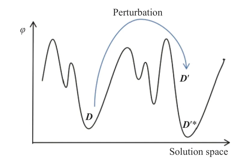
Fig.1 ILS

3.Iterated local coordinate-exchange algorithm

The flow chart of the iterated local coordinate-exchange algorithm for constructing experimental designs for multidimensional constrained spaces is shown in Fig.2.First of all, the initial designDis given and set as the current optimal solution.Then it is optimized by the local search algorithm, the optimized solution is obtained, and the current optimal solutionDis updated.Because the current optimal solutionDmay be a locally optimal solution, it is necessary to apply perturbation to make it “jump out” of the local area.The perturbed solution according to the perturbation strategy (including the perturbation object and the perturbation type) is recorded asD', and it is also optimized by the local search algorithm.The local search and perturbation are repeated, and finally the optimal solution is returned after the number of iterations is reached.

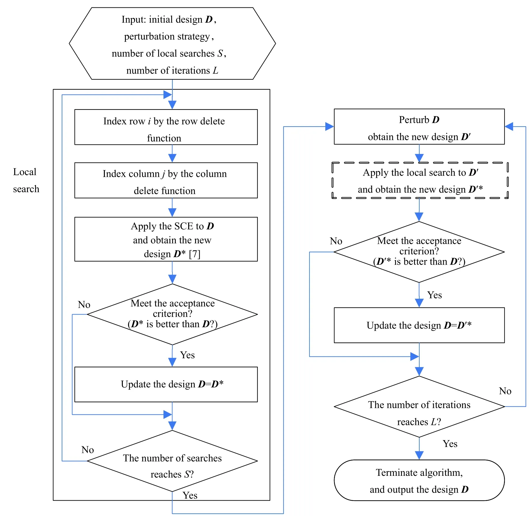
Fig.2 Flow chart of the iterated local coordinate-exchange algorithm

The pseudo code of the ILS algorithm is as follows:

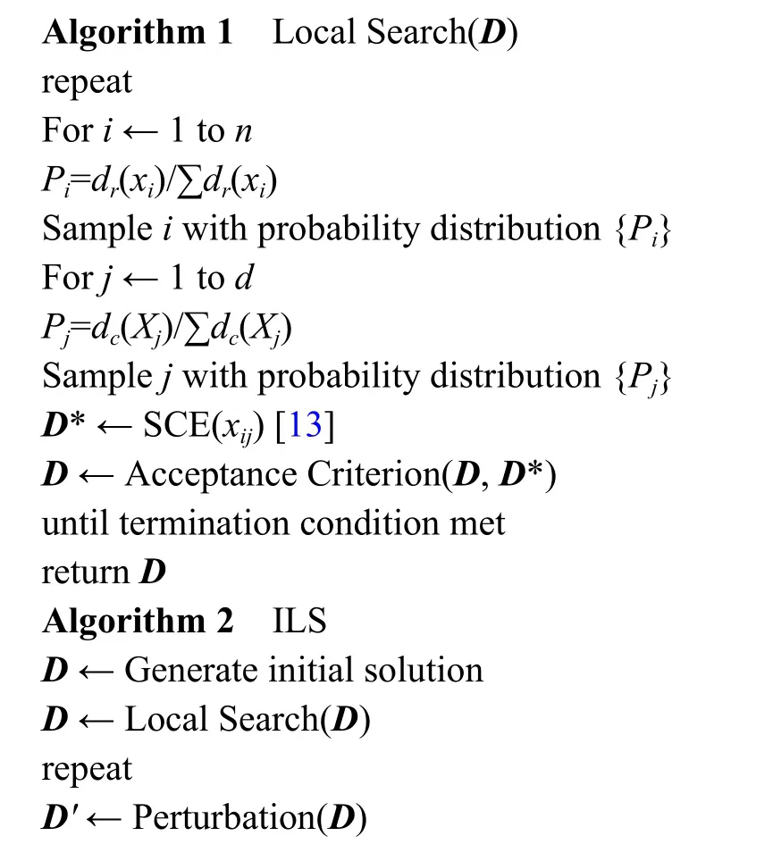
Algorithm 1 Local Search(D)repeat For i ← 1 to n Pi=dr(xi)/∑dr(xi)Sample i with probability distribution {Pi}For j ← 1 to d Pj=dc(Xj)/∑dc(Xj)Sample j with probability distribution {Pj}D* ← SCE(xij) [13]D ← Acceptance Criterion(D, D*)until termination condition met return D Algorithm 2 ILS D ← Generate initial solution D ← Local Search(D)repeat D' ← Perturbation(D)

D'* ← Local Search(D')D ← Acceptance Criterion(D, D'*)until termination condition met return D

3.1 Initial design

In this paper, a random number generator is used to construct the initial design.First, a single or a batch of points are uniformly sampled from the unconstrained space(xmin,xmax), and whether they meet all the constraints is checked.Accept points that satisfy all constraints and reject points that do not.Repeat the sampling and“reject/accept” steps untilndesign points are obtained.The calculation of the construction of initial design mainly depends on the number of points to be sampled and the percentage of the constraint space in the whole space (xmin,xmax).Some more complex methods may return higher quality initial design, but may take more running time under complex constraints, and it is pointed out in [13] that local search algorithms such as the coordinateexchange algorithm are not very sensitive to the quality of the initial design, where only the initial design is needed to meet the constraints.Therefore it is feasible to use the random sampling method for constructing initial design.

3.2 Local search

The potential power of ILS lies in the biased sampling of the set of local optima, and the efficiency mainly depends on the perturbation and the acceptance criterion.However, if the module of local search is optimized, a better performance can be obtained [25].Experiments have shown that applying more frequent and faster local search algorithms may be more effective than applying more powerful but slower ones [15,26?28].coordinatewhich may improve the design criterion.

Considering the applicability to the constrained space,this paper uses the SCE algorithm proposed by Kang [13]as the local search strategy: the coordinates to be exchanged in the design matrixDare selected with a probability proportional to the “delete function”.The delete function is used to evaluate which rows and columns can bring the greatest improvement, as defined in [13], and the rest of the coordinatesxil(l≠j) remains unchanged.The values ofxilare substituted into the linear or nonlinear equations or inequalities that define the constraints and solve them with respect toxij.That is, project theddimensional constrained design space to thejth input dimension and solve the 1-dimensional optimization problem for the projection area, in order to find the optimal

3.3 Perturbation strategies

The main goal of this stage is to jump out of the local optimal area by perturbing the current local optimal solution.

When using the ILS algorithm, the size of the perturbation is one of the most important problems.If the perturbation is too small, it will usually fall back to the local optimal solution of the previous step, so it is almost impossible to explore a new solution space.On the other hand, if the perturbation is too large, it may increase the running time and even lead to an effect similar to the random restart search.

Here we first propose several feasible perturbation objects and perturbation types.The perturbation object can be the design points or the coordinates of the design points.Point perturbation first selects the design points to be perturbed, and exchanges these design points with new design points that meet the constraint conditions.Coordinate perturbation first selects the coordinates of the design points to be perturbed, and exchanges these coordinates with new feasible coordinates that meet the constraint conditions.The type of perturbation can be deterministic or random.The deterministic type is to select the “worst” design points or coordinates of the current optimal solution and the random type is to select design points or coordinates randomly.

Through experiments, it is found that when the proportion of the perturbed points or coordinates to the total design is too large, it will destroy the relative structure of the current optimal solution, which is detrimental to the performance of the algorithm, so the perturbation object described below refers to one design point or one coordinate of a design point.

3.4 Acceptance criterion

The acceptance criterion determines whether to accept the new solution as the current optimal solution.Acceptance criterion has a strong influence on the nature and effectiveness of the search in the solution space.In a way, together with perturbation, the procedure controls the balance between intensification and diversification of the search [26].We can consider the strategy of improvement type ascent (or descent): for example, acceptD′*whenψ(D′*)＞ψ(D), that is, letD=D′*.Another strategy is to accept the new solution regardless of whether improvement is mad or not: for example, directly letD=D′*.Other strategies can also be considered, depending on the specific problem.

In this paper, the improvement type ascentψ(D) and the improvement type descent φpare taken as the acceptance criteria respectively, and these two criteria are taken as the target in the following example analysis and comparison.

4.Statistical analysis of parameters

The analysis of the iterated local coordinate-exchange algorithm shows that the main parameters affecting the performance of the algorithm include the number of local searches, the number of iterations, the perturbation object, and the perturbation type.This section studies the influences of these parameters on the performance of the algorithm and the interactions of these parameters through sensitivity analysis.

Select the different levels of the above four parameters,see Table 1, and use JMP program to generate several combinations of parameter levels.Taking example 3 in[13] as an example, setn=20, and the value of φpis calculated as the response of the experiments.

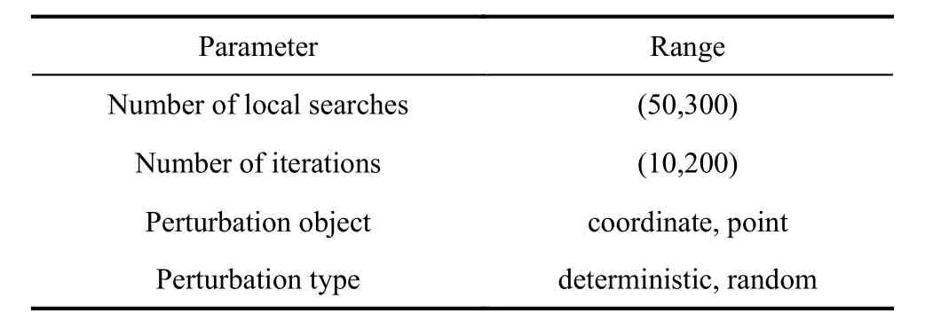
Table 1 Parameters and ranges

Since the iterated local coordinate-exchange algorithm is stochastic in nature, heteroscedasticity or variance of the variability, may exist in the raw data.Ignoring it may bias the standard errors andpvalues, and possibly weaken the analysis [29].In order not to core information, the mean value of 30 repeated observations at each design point is calculated as the response value of each design point.The scheme and the experimental results are shown in Fig.3.

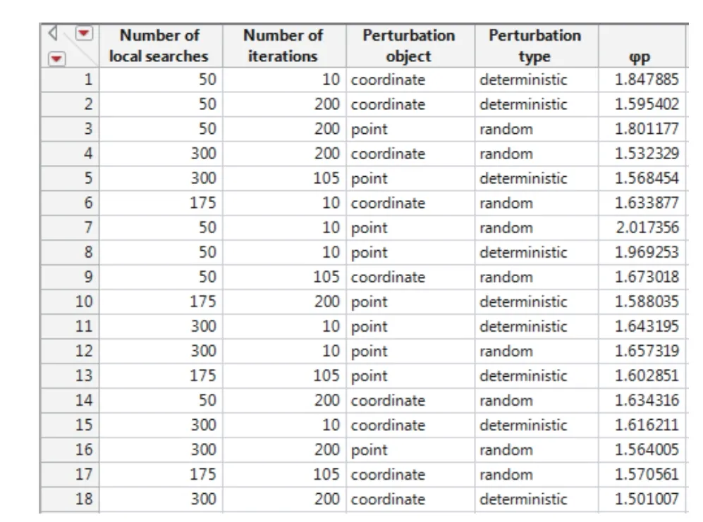
Fig.3 Design scheme

Fig.4 shows the histogram, box plot, and quantiles of the response values of all experiments.The median is 1.625 and the upper quartile is 1.705.Compared with the running result 1.731 of the SCE algorithm with 300 local searches and 200 iterations, it can be seen that even under poor operating conditions, the proposed algorithm in this paper makes a great improvement on the random restart SCE algorithm.The two outliers are the combination of 50 searches and 10 iterations.Note that each outlier is not a single observation, but the mean of 30 observations.This indicates that the local search may stop and proceed to the next iteration before the local optimal solution is reached, resulting in the failure to explore the better solution.

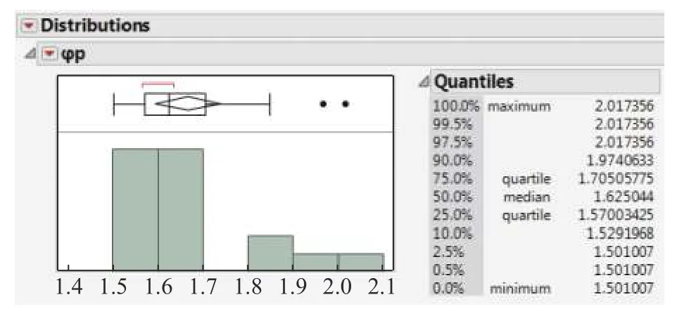
Fig.4 Distribution

The regression tree shown in Fig.5 shows that the number of local searches is important, and multiple searches may help to reach a better solution.The second split occurs on the parameter of the perturbation object,when the perturbation object is “coordinate”, the mean of responses is 1.571, and when the perturbation object is“point”, the mean of responses is 1.604.This shows that the selection of the perturbation object will also have a great impact on the performance of the algorithm, and a big perturbation may destroy the characteristic structure of the current optimal solution.

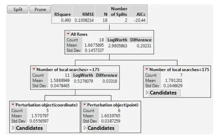
Fig.5 Regression tree

A fitted model is established through a stepwise regression.The fitted model withR2equal to 0.81 is obtained without interaction, as shown in Fig.6(a).Performing a multiple regression with interactions between factors raisedR2to 0.99, suggesting an improved fitted model.By observing the F-test results in Fig.7, the fitting and parameter estimation are complementary to the regression tree.From the ranking ofFratio, we can also see the importance of the number of local searches, the number of iterations, the perturbation object and their interactions.When the perturbation type is “deterministic”,the performance of the algorithm is slightly improved, but the complexity of the algorithm is increased, so it is suggested that the perturbation type be set to “random” in order to reduce the running time and improve the computational efficiency.If there is a higher requirement for accuracy, the perturbation type can be set to “deterministic”,depending on the specific demands.

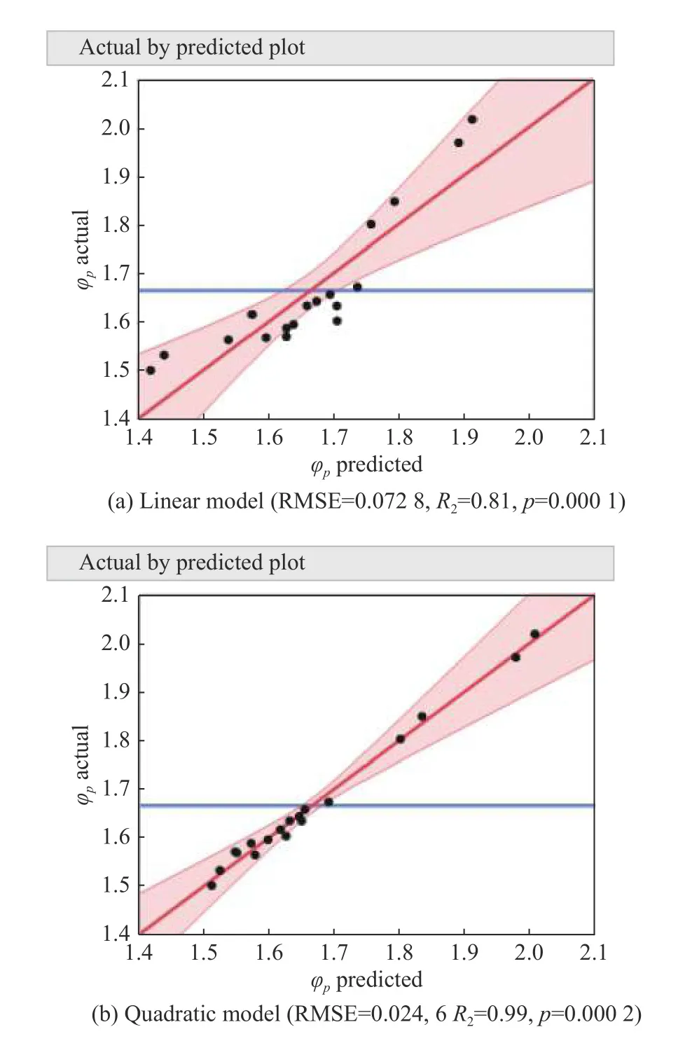
Fig.6 Model fitting

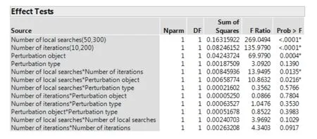
Fig.7 Effect test

Continuing the analysis, we use parameters that have a significant impact on the response to fit the model, and focus on the analysis of the number of local searches, the number of iterations, the perturbation object and their interactions.As can be seen from Fig.8, there is a significant interaction between the number of local searches and the perturbation object, as well as the number of local searches and the number of iterations.When the number of local searches is small, the increase of the number of iterations and the reasonable selection of the perturbation object have obvious effects on the improvement of response φp.The setting of the perturbation object to “coordinate” will be more conducive to the exploration of a better solution.For the local search algorithm, too few times of local search will not find the local optimal solution, but when the number of searches is about 200, continuing to increase the number of searches will not help to improve the value of φp, on the contrary, it will increase running time of the algorithm.The number of iterations and the number of local searches complement each other to some extent.

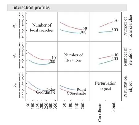
Fig.8 Interaction

Through the above experiments, it is found that the number of local searches and the number of iterations may complement each other.In order to further explore the relationship between them, experiments are carried out on the different level combinations of the number of local searches and the number of iterations.The perturbation object is fixed as “coordinate” and the perturbation type is fixed as “random” .The number of iterations is expressed byL, the number of local searches is expressed byS, and the product ofLandSrepresents the total number of operations.The experimental results are shown in Fig.9, the point graph from top to bottom are the response values corresponding to the total operations of 10000, 20000, and 30000.The ordinate of Fig.9 is the response value φp.and the abscissa is the different combinations of the number of local searches and the number of iterations, expressed by.Similarly, each point is the mean of 30 repeated observations.It can be seen that whenL×Sincreases, the response value increases accordingly.WhenL×Sis the same, changing the combination ratio of the number of local searches and the number of iterations has little effect on the results.However, when the ratio is too wide, such as few iterations or few local searches, it will have an adverse effect on the response value.The overall performance of the algorithm is stable with the response value between 1.53 and 1.58.If you want to get a better response value, you can achieve it by increasing the total number of operations, and it is recommended that the number of iterations and the number of local searches should not be set too low.

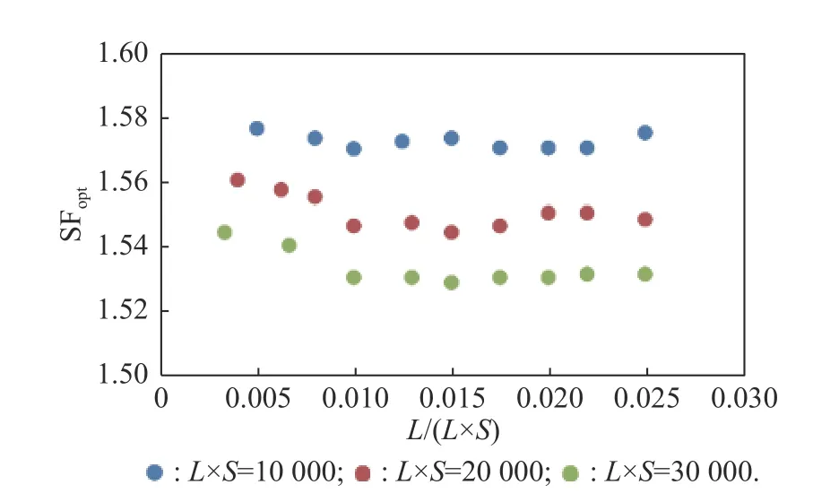
Fig.9 Number of iterations and number of searches

The above conclusions are also valid for the D-optimal criterion.The specific simulation experiment data and process are not given due to the limited space.

Based on the results of parameter sensitivity analysis,in order to reduce the running time and improve the search efficiency, we suggest to select “coordinate” as the perturbation object, and select “random” as the perturbation type, and set a reasonable combination of the number of local searches and the number of iterations according to the demand.In the next example analysis, the total number of operations is set to 20000, where the number of iterations is set to 100 and the number of local searches is set to 200.

5.Example analysis

In example 2 of [13], it is assumed that a constraint is

forx1,x2∈[0,1]2, forming a 2-dimensional non-convex design space.Set the number of runsn=20, the number of local searchesS=200, and the number of iterationsL=100.The optimal values returned by the algorithm proposed in this paper and the SCE algorithm are 4.786 and 6.399 respectively, as shown in Fig.10.Setn=40 and use the same quadratic model as Kang [13], Fig.11 shows the D-optimal and the φp-optimal values returned by our algorithm and the SCE algorithm with different number of local searches.The ordinates of Fig.11(a), Dopt, and that of Fig.11(b), SFopt, correspond to the response value (D)and the response value φp, respectively, and the abscissa is the number of local searches.It can be seen that in the 2-dimensional constrained space, the algorithm proposed in this paper performs better under both D-optimal and φp-optimal criteria, while the SCE algorithm does not perform well when the number of local searches is low,especially when D-optimal is taken as the goal.By increasing the number of local searches and restart times,the SCE algorithm can also obtain desired design results.At the same time, it can be seen that the algorithm proposed in this paper is relatively stable and insensitive to the number of local searches, and the desired optimal design can be obtained even with a small number of local searches, which is of significance to save running memory, reduce running time and improve search efficiency.

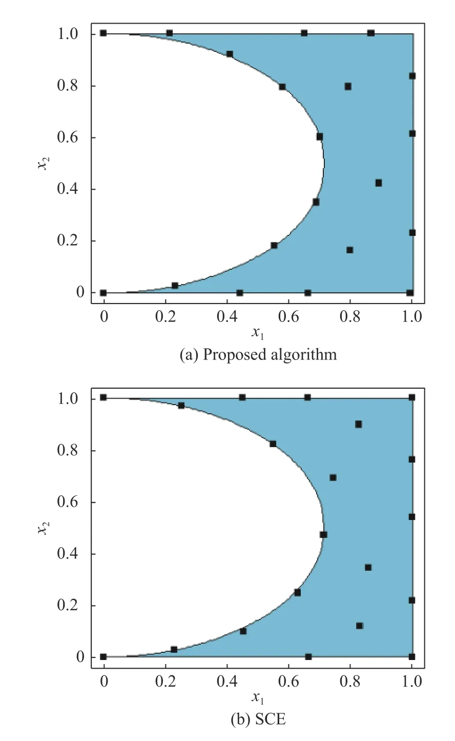
Fig.10 Comparison of design schemes (n =20)

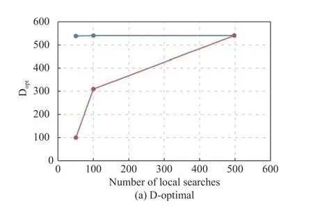
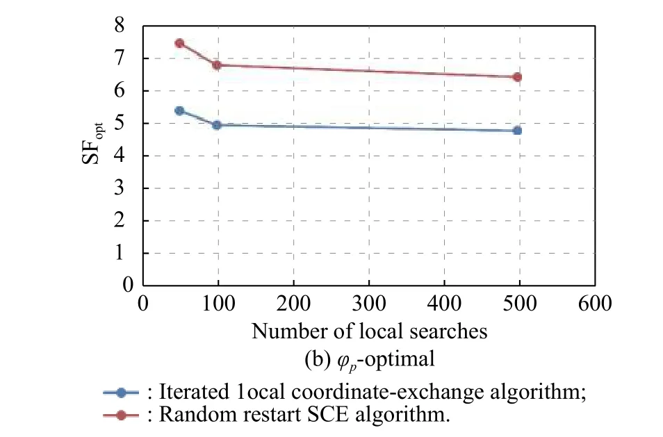
Fig.11 Algorithm comparison in two-dimensional non-convex constrained space

Let us take a look at the performance of the two algorithms in high-dimensional constrained space, a real case of a total elbow replacement computer simulation[30] is illustrated.This experiment involves four factors,and the constraints are as follows:

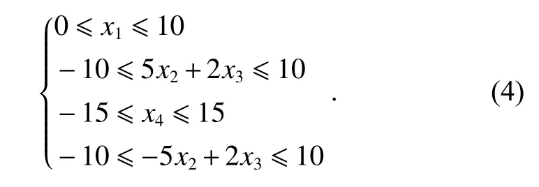
Set the number of runsn=10 and the number of iterationsL=100, the D-optimal and the φp-optimal values returned by the algorithm proposed in this paper and the SCE algorithm with different number of local searches are shown in Fig.12.It can be seen that the algorithm proposed in this paper also performs better than that of the SCE algorithm in 4-dimensional constrained space,especially under the D-optimal criterion.The SCE algorithm cannot reach the desired value either by increasing the number of searches or restart times.The SCE algorithm shows a larger gap with our algorithm in 4-dimensional constrained space.However, the proposed algorithm also performs generally in the D-optimal design with low number of local searches, so it is necessary to increase the number of local searches or iterations to improve the design quality.

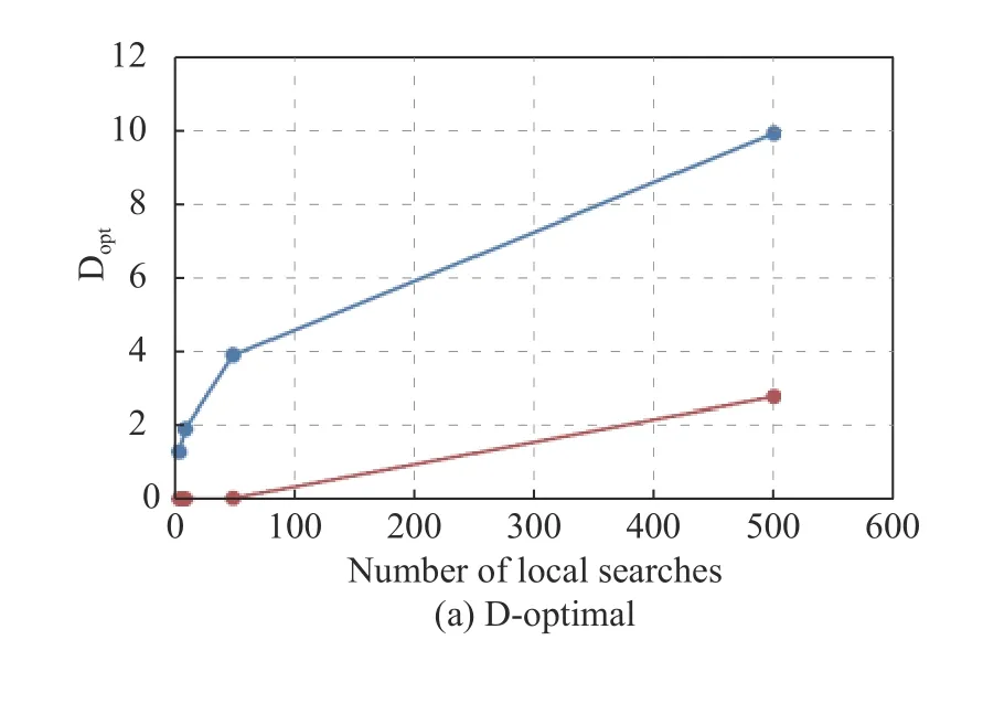
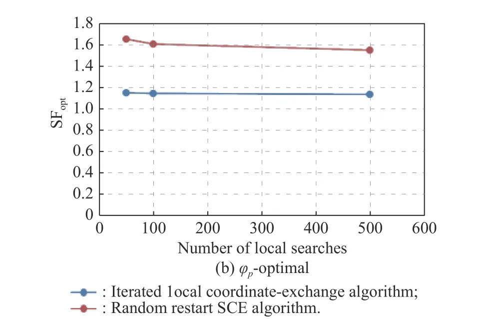
Fig.12 Algorithm comparison in 4-dimensional constrained space

6.Conclusions

The SCE algorithm reduces the execution time by transforming the problem of finding the optimal coordinate into exploring the 1-dimensional optimal solution, and it reduces the possibility of falling into the local optimal solution by selecting coordinates stochastically.However,just like the “hill climbing” method, only coordinate-exchange that makes improvement will be considered in each iteration, resulting in low possibility of exploring a better solution.Therefore, a new iterated local coordinateexchange algorithm is proposed to optimize the experimental design, and the sensitivity analysis is conducted to identify the parameters that have a significant impact on the performance of the algorithm.Through the comparison of experiments with different dimensions, parameter settings and optimization goals, it is shown that the proposed iterated local coordinate-exchange algorithm is better than the SCE algorithm using the random restart strategy in improving the running efficiency and optimizing the design quality, especially in the experimental design for high-dimensional constrained space.Applying this method, it is suggested that the perturbation object should be set to “coordinate” and the perturbation type should be set to “random”.If there is a higher requirement for precision, the perturbation type can be set to“deterministic”, and the total number of operations can be set higher.Meanwhile, either the number of iterations or the number of local searches should not be set too low.