JIAO Dan

(School of Electrical and Computer Engineering, Purdue University, West Lafayette， Indiana 47907, USA)

Abstract:In this paper, we demonstrated a fast direct finite-element solver of linear (optimal) complexity for analyzing large-scale system-level interconnects and their related signal and power integrity problems. This direct solver had successfully analyzed an industry product-level package and correlated with measurements in time domain. The finite-element matrix of over 15.8 million unknowns resulting from the analysis of the industry package, including both signal lines and power delivery structures, was directly solved in less than 1.6 h on a single core running at 3 GHz. Comparisons with the state-of-the-art finite element methods that employed the most advanced direct sparse solvers, and a widely used commercial iterative finite element solver, had demonstrated the clear advantages of the proposed linear-complexity direct solver in computational efficiency.

Keywords: finite-element method; signal and power integrity; time-domain method

0 Introduction

With the increase in the processing power of the CPU, the memory and system interconnect links connected to a CPU need to have an exponentially increased bandwidth in order to fully utilize the computing power. This leads to higher speed signals on each data line as well as an increase in the number of data lines. Enabling higher bandwidth brings significant challenges to the analysis and design of interconnects. To address these challenges, a full-wave modeling technology is required that can rapidly characterize the interaction between a large number of I/Os in the face of large problem sizes.

Existing fast full-wave solvers for solving large-scale problems are, in general, iterative solvers since traditional direct solvers are computationally expensive. The optimal complexity of an iterative solver isO(NrhsNitN), whereNrhsis the number of right hand sides,Nitis the number of iterations, andNis the matrix size. To analyze the interaction among a large number of circuit ports and to perform many what-if analyses for an optimal design, the number of right hand sides is proportional to the port count and the number of what-if analyses. When the number of right hand sides is large, iterative solvers become inefficient. In contrast, a direct solver has a potential of achievingO(N) complexity, which is optimal for solvingNunknowns.

Among existing full-wave solvers, the finite element method (FEM) is a popular method for analyzing circuits because of its great capability in handling both complicated materials and geometries. A traditional direct finite element solver is computationally expensive. It is shown in Ref.[1] that the optimal operation count of a direct FEM solution in exact arithmetic isO(N1.5) for 2-D problems, andO(N2) for 3-D problems. Although there have been successes in speeding up the direct finite element solution with state-of-the-art sparse matrix solvers[2-4], these solvers have not accomplishedO(N) complexity, i.e., optimal complexity, for FEM-based direct solutions of general 3-D circuit problems.

In recent years, we have successfully achieved the first direct finite-element solver of linear complexity[5-6]. This solver is capable of analyzing arbitrarily shaped 3-D circuits in inhomogeneous materials. An IBM product-level package problem[7]having over 15.8 million unknowns is directly factorized and solved for 40 right hand sides in less than 1.6 h on a single 3 GHz CPU core. The signal integrity of the package interconnects in presence of the surrounding power delivery network is analyzed. Excellent correlation with the measured data is observed. In addition, we have compared the proposed direct solver with a suite of state-of-the-art high-performance direct sparse solvers such as MUMPS 4.10.0[2], and Pardiso in Intel MKL[4]. It is shown that the proposed direct solver greatly outperforms state-of-the-art sparse solvers in both CPU time and memory consumption with good accuracy achieved.

1 Vector finite element method and mathematical background

1.1 Vector finite element method

Considering a general physical layout of a package or integrated circuit involving inhomogeneous materials and arbitrarily shaped lossy conductors, the electric fieldEsatisfies the following second-order vector wave

(1)

whereμris relative permeability,εris relative permittivity,σis conductivity,k0is free-space wave number,Z0is free-space wave impedance, andJis current density. A finite element based solution of Eq. (1) subject to pertinent boundary conditions results in the following linear system of equations

YX=B,

(2)

whereY∈N×Nis a sparse matrix, and matrixBis composed of one or multiple right hand side vectors. When the size of Eq. (2) is large, its efficient solution relies on fast and large-scale matrix solutions.

1.2 Mathematical Background

In state-of-the-art direct sparse solvers, multifrontal method[2]is a powerful algorithm. In this algorithm, the overall factorization of a sparse matrix is organized into a sequence of partial factorizations of smaller dense frontal matrices. Various ordering techniques have been adopted to reduce the number of fill-ins introduced during the direct matrix solution process. The computational cost of a multifrontal based solver depends on the number of nonzero elements in theLandUactors of the sparse matrix. In general, the complexity of a multifrontal solver is higher than linear (optimal) complexity.

Recently, it is proved in Ref.[3] that the sparse matrix resulting from a finite-element based analysis of electromagnetic problems can be represented by anH-matrix[8]without any approximation, and the inverse as well asLandUof this sparse matrix has a data-sparseH-matrix approximation with a controlled error. In anH-matrix[8], the entire matrix is partitioned into multilevel admissible blocks and inadmissible blocks. An inadmissible block keeps its original full matrix form, while an admissible block is represented by an error-controlled low-rank matrix. It is shown in Ref. [3] that anH-matrix based direct FEM solver has a complexity ofO(NlogN) in storage and a complexity ofO(Nlog2N) in CPU time for solving general 3-D circuit problems.

2 Proposed linear complexity direct fem solver for large-scale interconnect extraction and related signal and power integrity analysis

2.1 Proposed direct solver

In the proposed solver, we fully take advantage of the zeros in the original FEM matrix, and also maximize the zeros inLandUby nested dissection ordering[1]. We store the nonzero blocks inLandUwith a compact error-controlledH-matrix representation, compute these nonzero blocks efficiently by developing fastH-matrix based algorithms, while removing all the zeros inLandUfrom storage and computation. Moreover, we organize the factorization of the original 3-D finite element matrix into a sequence of factorizations of 2-D dense matrices, and thereby control the rank to follow a 2-D based growth rate, which is much slower than a 3-D based growth rate[9]for analyzing circuits operating at high frequencies. The overall algorithm has six major steps:

(1) Build cluster treeTIbased on nested dissection;

(2) Build elimination treeEIfromTI;

(3) Obtain the boundary for each node inEI;

(4) Generate theH-matrix structure for each node;

(5) Perform numerical factorization guided byEIby new fastH-matrix-based algorithms;

(6) Solve for one or multiple right hand sides based onEI.

To build cluster treeTI, we recursively partition a 3-D computational domain into separators and subdomains. Since a separatorScompletely separates two subdomainsD1andD2, the off-diagonal blocks in the FEM matrix corresponding to the interaction betweenD1andD2, denoted byYD1D2andYD2D1, are zero. More important, the same zero blocks can be preserved in theLandUfactors.

The LU factorization of the FEM matrix is a bottom-up traversal of the elimination tree as that used in the multifrontal algorithm. Note that the union of all the nodes inEIis equal to I, which is different from cluster treeTI. For each nodesin the elimination tree, we assemble a frontal matrixFsfrom the system matrixYand all the updating matricesUcwithc∈Esbeings’s children nodes. TheFscan be written as a 2×2 block matrix

(3)

in whichΦsdenotes the boundary ofs. We then apply partial LU factorization toFs, obtaining

(4)

Comparing Eq. (3) and (4), we can readily obtain the updating matrixUs

Us=FΦs,Φs-LΦs,sUs,Φs,

(5)

which is then used for the LU factorization of the frontal matrices ofs’s ancestors inEI. The entire LU factorization of matrixYis a bottom-up or post-order traversal ofEI. ForΦs, we have an important lemma

(6)

Therefore, minimizing#{Φs}, the size ofΦs, is critical in avoiding unnecessary operations on zeros. We thus first perform symbolic factorization to pre-process the elimination tree to compute the minimumΦsfor each node inEIbefore the real factorization is carried out.

2.2 Complexity and accuracy analysis

(7)

(8)

which is linear. The accuracy of such anH-matrix representation can be proved from the fact that the original FEM matrix has an exactH-representation and its inverse has an error-boundedH-representation[3].

3 Performance demonstration

3.1 Intel package interconnect with measured data

A 3-D package interconnect provided by Intel Corporation is simulated from 50 MHz to 40 GHz. Fig.1A illustrates the cross sectional view, top view, and 3-D view of the package interconnect. In Fig.1B and Fig.1C, we plot theS-parameters extracted by the proposed solver in comparison with the measure data and the results generated from a commercial FEM-based tool. Excellent accuracy of the proposed solver can be observed in the entire frequency band.

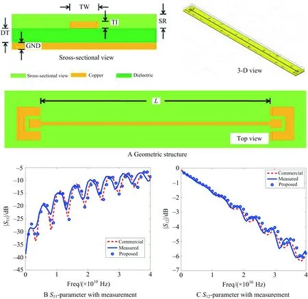
Fig.1 Simulation of a realistic Intel package interconnect example and correlation with measurements

3.2 IBM full-package problem with measurements

An IBM product-level package[7]is simulated from 100 MHz to 50 GHz to examine the capability of the proposed direct finite element solver. The package involves 92 thousand unique elements. There are eight metal layers and seven dielectric layers. We develop software to interpret the board file of the full IBM package into the geometrical and material data that can be recognized by the proposed solver, and also mesh the entire layout of the package into triangular prism elements. The layout of selected layers re-produced by our geometrical processing software can be seen from Fig.2.

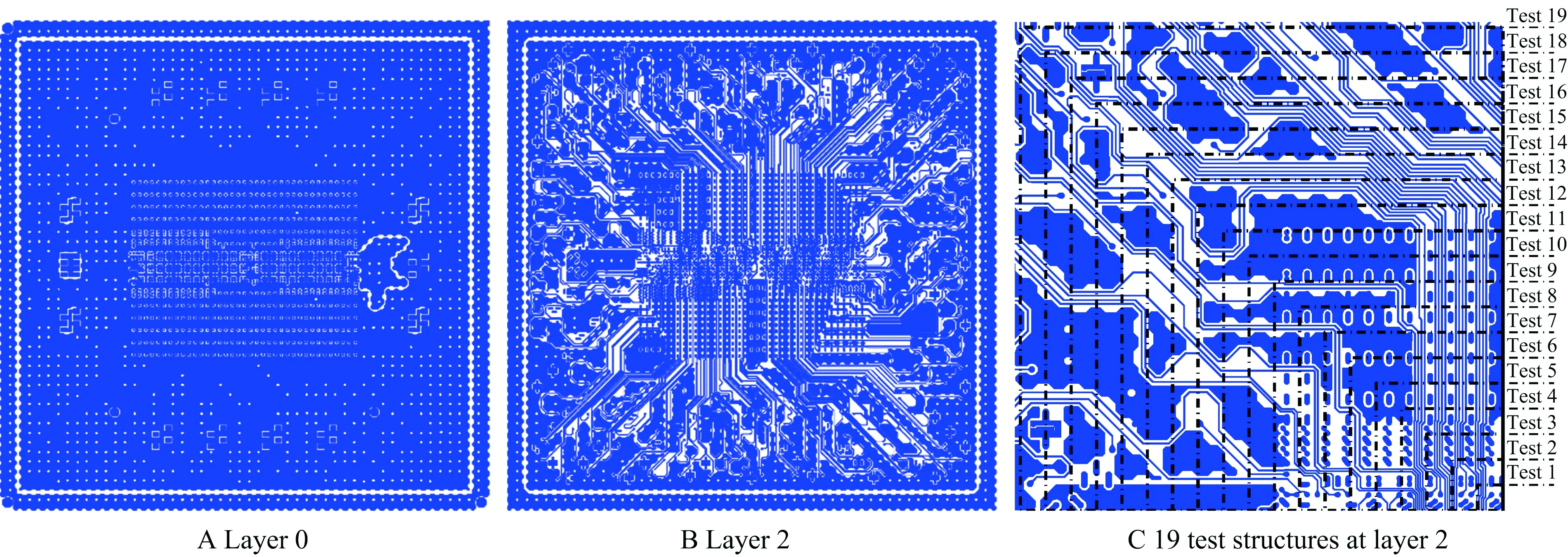
Fig.2 Layout of a product-level package in different layers and 19 test structures for solver performance verification

3.2.1 Complexity and performance verification

To examine the accuracy and efficiency of the proposed direct solver, a suite of nineteen substructures of the full package is simulated. These substructures are illustrated in Fig.2C. The smallest structure occupies a package area of 500 μm in width, 500 μm in length, and 4 layers in thickness, whereas the largest structure occupies a package area of 9 500 μm by 9 500 μm. The resultant number of unknowns ranges from 31 276 to 15 850 600. Two ports at the topmost layer are excited. The important simulation parameters used in the proposed direct solver are leafsize=8 and truncation error ∈=10-6. The computer used has a single core running at 3 GHz with 64 GB memory.

The CPU time and memory cost of the proposed solver with respect to unknown numberNare shown in Fig.3 in comparison with those of the direct finite element solver that employs the most advanced direct sparse solvers provided by SuperLU 4.3, UMFPACK 5.6.2, MUMPS 4.10.0[2], and Pardiso in Intel MKL[4]. It is evident that the proposed direct finite element solver greatly outperforms the other state-of-the-art direct solvers in both CPU time and memory consumption. More important, the proposed direct solver demonstrates a clear linear complexity in both time and memory across the entire unknown range, whereas the complexity of the other direct solvers is much higher. With the optimal linear complexity achieved, the proposed direct solver is able to solve the extremely large 15.8 million unknown case using less than 1.6 h on a single core. The solution error of the proposed direct solver, measured in relative residual, is plotted in Fig.3C for all of the testing cases. Excellent accuracy is observed across the entire unknown range. Note the last point in Fig.3B is due to the fact that the computer used has only 64 GB memory.

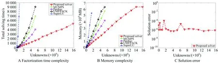
Fig.3 Complexity and performance verification of the proposed direct solver

3.2.2 Signal and power integrity analysis and correlation with measurements

With the accuracy and efficiency of the proposed direct solver validated, next, we analyze the signal and power integrity of the IBM product-level package and correlate our analysis with measured data. First, the frequency-domain S-parameters from 100 MHz to 30 GHz were generated for 16 ports assigned to 2 interconnects located in the full package. The near-end ports are placed on the topmost layer (chip side), while the far-end ports are at the bottom-most layer (BGA side). The entire stack of 8 metal layers and 7 inter-layer dielectrics are simulated. The resultant number of unknowns is 3 149 880.

The proposed direct solver only takes less than 3.3 h and 29 GB peak memory at each frequency to extract the 16 by 16S-parameter matrix, i.e. solutions for 16 right hand sides. The crosstalk between the near end of line 6 (port 9) and the far end of line 2 (port 8) with all the other ports left open is plotted in Fig.4 from 100 MHz to 30 GHz. The measurement of the structure is performed in time domain[7]. As shown in Fig.4C, very good agreement is observed between the time-domain voltage obtained from the proposed solver and the measured data.

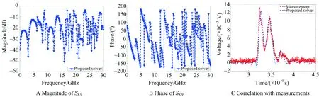
Fig.4 Time domain correlation with measurements

4 Conclusion

In this paper, we develop a linear-complexity direct finite element solver to analyze large-scale interconnects and related system-level signal and power integrity problems. Comparisons with measurements and state-of-the-art sparse solvers have demonstrated the superior performance of the proposed direct solver in accuracy, efficiency and capacity.