Min WAN ,Wan-Jing XING ,Yang LIU ,Qun-Bao XIAO ,Wei-Hong ZHANG

a School of Mechanical Engineering,Northwestern Polytechnical University,Xi'an 710072,China

b State IJR Center of Aerospace Design and Additive Manufacturing,Northwestern Polytechnical University,Xian 710072,China

KEYWORDS Energy approximation method;Error-controllable global smoothing method;G3 continuity;Local smoothing method;Quasi-uniform quintic Bspline curve

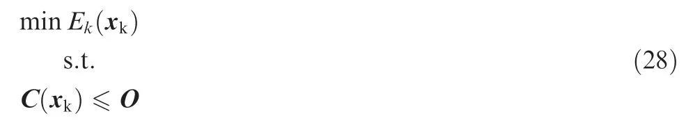
Abstract In real machining,the tool paths are composed of a series of short line segments,which constitute groups of sharp corners correspondingly leading to geometry discontinuity in tangent.As a result,high acceleration with high fluctuation usually occurs.If these kinds of tool paths are directly used for machining,the feedrate and quality will be greatly reduced.Thus,generating continuous tool paths is strongly desired.This paper presents a new error-controllable method for generating continuous tool path.Different from the traditional method focusing on fitting the cutter locations,the proposed method realizes globally smoothing the tool path in an error-controllable way.Concretely,it does the smoothing by approaching the newly produced curve to the linear tool path by taking the tolerance requirement as a constraint.That is,the error between the desired tool path and the G01 commands are taken as a boundary condition to ensure the finally smoothed curve being within the given tolerance.Besides,to improve the smoothing ability in case of small corner angle,an improved local smoothing method is also proposed by symmetrically assigning the control points to the two adjacent linear segments with the constrains of tolerance and G3 continuity.Experiments on an open five-axis machine are developed to verify the advantages of the proposed methods.

1.Introduction

Most of complex parts such as thin-walled workpieces are machined by CNC milling process.1-3Although modern CNC controllers are capable of dealing with tool paths in the form of splines,complex parts are often machined by post-processing the tool paths as a series of short linear segments,i.e.G01 command in most modern CAD/CAM software.4-6As shown in Fig.1,the short linear segments are connected by sharp corners,which can cause the discontinuity of tangential velocity in machining.7This phenomenon will result in the infinite acceleration and jerk,and thus damage the machine tools.In the worst case,limited by the finite acceleration and jerk of machine tools,the tool motion has to be stopped at every corner and restart.This will lead to a greatly increased time consume and a poor surface. Reasonably smoothing the tool paths with corners can ensure continuous and steady motion,and thus guarantee the machining accuracy.There are two main methods to smooth the tool path,i.e.local corner smoothing method and global corner smoothing method.

The local corner smoothing method is realized by inserting a micro-Spline curve to approximate the linear segments at each corner.A review of literature shows that there are local smoothing methods for three-axis machining8-11,7,12and for five-axis machining,13-18respectively. Pateloup et al.8and Zhao et al.10employed a cubic B-spline to smooth the corner between two adjacent lines for the tool path of three-axis milling.Sencer11smoothed the local corner by inserting a quintic Bezier curve,and minimized the spline curvature to ensure G2 continuous motion transition between linear segments.Beudaert et al.13used two cubic B-spline curves to represent the five-axis tool paths,and then smoothed the tool tip positions and tool orientation.Jin et al.15also proposed a dual-Bezier path smoothing algorithm for five-axis machining,and used double G2 continuous cubic Bezier curves to smooth tool tip position and orientation.Farouki14did this by using seven degree Pythagorean Hodograph curves.Tulsyan and Altintas16proposed a decoupling algorithm for tool tip position and orientation of five-axis tool paths,and employed a quintic and a 7th B-spline curves to smooth the tool tip position and orientation to ensure the G3 continuity.Based on Tulsyan and Altintas's work,Yang et al.17and Hu et al.19proposed analytical local corner smoothing algorithms for fiveaxis and four-axis CNC machine tools,respectively.It should be pointed out that the local smoothing methods of tool tip position for five-axis machining are similar to those related to three-axis machining.The traditional local smoothing methods are beneficial to improve the smoothness of the G01 tool path,however,problems still exist.Part of the local smoothing methods can only achieve G2-continuity,and such trajectories cannot ensure the continuity of jerk.The other part cannot achieve the optimal curvature of the inserted B-spline,which will lower the cutting speed.The aforementioned problems can be both solved by adopting the local and global smoothing methods proposed in this article.

There also exist a kind of methods,named global corner smoothing methods,fit all desired cutter locations to spline representations.For three-axis CNC machining,quintic polynomial spline20and NURBS curve21,22were usually used to fit the tool paths. Whereas, for five-axis CNC machining,decoupled-spline23is used to fit the tool paths.Lei et al.21proposed a fast real-time NRUBS path interpolation method to generate the tool path.Heng and Erkokmaz22presented a robust and numerically efficient NURBS interpolation to fit tool paths of three-axis machining,and avoided the unwanted feed fluctuations and sensitivity to round-off errors by applying the feed correction polynomial concept to NURBS tool paths in an adaptive manner.Yuen et al.23proposed a smooth spline interpolation technique for five-axis machining,and a quantic G3 B-spline was fitted by assigning control points and knots to force the spline passing through the tool tip position data.In summary,the global method mentioned above can guarantee the smoothness of tool path,however,they are difficult to control the accuracy of smoothed curve between the two adjacent cutter locations.

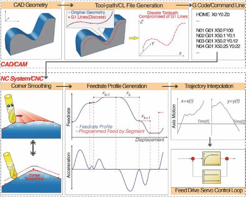
Fig.1 Sketch of one kind corner smoothing scheme7.

Hence, this paper proposes a new global smoothing method,which builds a global curve to approach the linear tool path rather than to fit the cutter locations.By doing this,it aims at both the smoothness and accuracy of tool path.Section 2 details the new global smoothing method,which is established based on a quinic B-spline curve.The generated curve can both guarantee the smoothness and respect the corner position tolerance.To be a necessary and beneficial supplement of the global method,an improved local smoothing method is also described in Section 2,in which a symmetrical quinic quasi-uniform B-Spline is inserted into the two adjacent linear segments to ensure the G3 continuity.The advantages of the proposed methods are experimentally verified on an open CNC experimental machine,as described in Section 3.

2.Smoothing of tool path with linear segments

2.1.the establishment of criterion

If a tool path has a series of tool tip position points pk(k=0,1,2,...,N),one can construct(N-1)number of local parts,and each part includes three adjacent points.The kth local part is constructed by points pk-1,pkand pk+1.For example,points p0,p1and p2constitute the first local part,while points p1,p2and p3constitute the second local part.Each part is treated as a local corner and the middle point is defined as a corner point.

As influenced by the length of linear segment,traditional local smoothing method may cause overlapping phenomenon.As shown in Fig.2,the red and yellow solid curves are the smoothed curves for the kth and(k+1)th corners respectively.They are not limited by length of line segment and the overlapping effect occurs.Once the overlapping effect occurs,the smoothed tool path is unreasonable.In this case,the smoothed tool path is still discontinuous and can result in the interruption of machining,which is difficult to be realized.Typical local smoothing methods solve this problem by scaling down the smoothed curve once the distance between the start/end point of smoothed curve and the corner point is larger than half of the location lined length.13,15-17,19This can lead to the increase of the curvature of the smoothed tool path.Fig.2 gives a schematic diagram to geometrically illustrate the overlapping effect.The thin solid and black dashed curves are the smoothed tool paths of the kth and(k+1)th corners after scaling down.It can be observed that the curves generated by the operation of scaling down have higher curvatures.To reduce the increase of curvature a new corner smoothing method is proposed.A criterion is established,based on which the whole tool path is divided into two categories with and without overlapping effect.

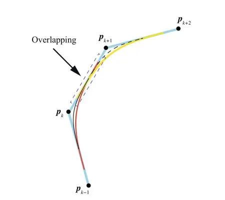
Fig.2 Overlapping effect occurring in local method.

The establishment of criterion is detailed as follows.The proposed local smoothing method uses a symmetrical Bspline with 7 control points to smooth the tool path(see Section 2.3),as shown in Fig.3.Symbol Pk,fis used to designate the fth control points of the smoothed curve for kth corner.Once overlapping effect occurs,the following equation can be obtained.

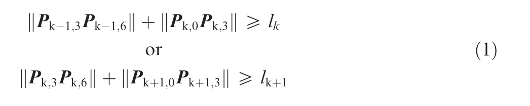
where lk=‖pk-pk-1‖.The whole tool path is divided into two categories with and without overlapping effect.The details on how to divide the tool path are described below.For a sequence of corners,the local smoothing method,which is proposed in Section 2.3,is used to generate the corresponding control points Pk,f.Then,using Eq.(1)judges whether overlapping effect occurs.For the control points of a corner satisfying Eq.(1),the corner is classified into the category with overlapping effect,called the first category.The remaining constitutes the second category.The sequential corners of the first category are smoothed by the global smoothing method,while each corner belonging to the second category is smoothed by the local smoothing method.It should be mentioned that after smoothing,the connections of the two tool path categories should satisfy the G3 continuity.Actually,this can be easily satisfied by reasonably choosing the first and last trajectory points of the line segments,which are needed by the global smoothing method.The first trajectory point used by the global smoothing method is chosen as the last control point of the former corner needed by the local smoothing method,while the last trajectory point used by global smoothing method is chosen as the first control point of the latter corner needed by the local smoothing method.Now,take Fig.4 as an example to illustrate how to classify the category.The whole tool path is divided into 7 parts and two categories.The parts 1,3,5 and 7 are the first category of corners needed by the global smoothing method,while the parts 2,4 and 6 are the second category of corners needed by the local smoothing method.A detailed explanation for the part 3 is given below.The first point of this part,which is not the corner point,is the last control point of the smoothed curve of the part 2,and the last point of the part 3 is the first control point of the smoothed curve of the part 4.That is,the line trajectory of the part 3 is the line connected by the first point,the corner points and the last point.Finally,it should be pointed out that if the category needing global smoothing occurs at the first part,the first point is the start point of the tool path,while if it occurs at the last part,the last point is the last point of the tool path.

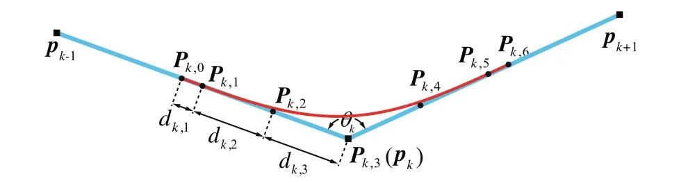
Fig.3 Symmetric quintic B-spline curve smoothed by local method for the kth corner.

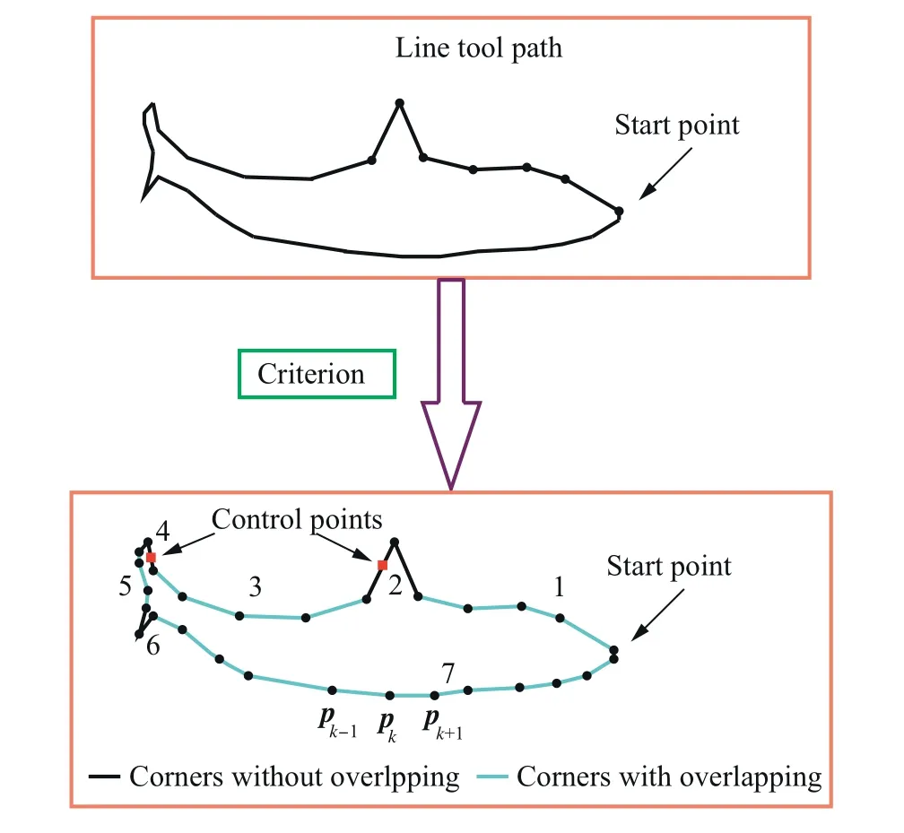
Fig.4 Classification of linear tool path.

2.2.Global smoothing method by considering tolerance requirement

In this section a quasi-uniform quintic B-spline curve is used to smooth the corners according to the procedure.Note that the brief introduction of B-spline curve is given in Appendix A.

2.2.1.Pre-smoothing of some corner points

In this section,the points of the tool path needed to conduct global smoothing are sequently marked as bj(j=0,1,2,...,M).Here,M+1 means the total number of tool tip position points.The control points of the global curve are marked as Bi(i=0,1,2,...,Q).Q+1 is the number of control points.To satisfy the G3 continuity at the junction points between the curve and the line,the first three and the last three control points can be defined as

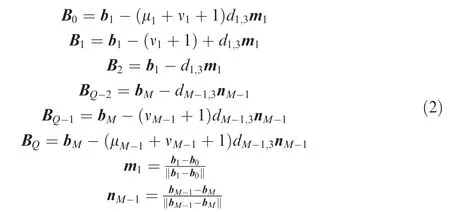
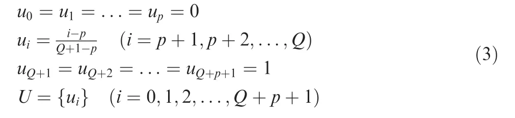
where μkand νkare defined as μk=dk,1/dk,3and νk=dk,2/dk,3.dk,1,dk,2and dk,3are the distances between the control points,which are required and defined related to the kth corner by the local method given in Section 2.3.As defined in Fig.3,dk,1is the distance between Pk,0and Pk,1.dk,2is the distance between Pk,1and Pk,2,and dk,3is the distance between Pk,2and Pk,3.It should be mentioned that the first three and the last three control points should inside the first and the last linear segment.Hence,if B0b1＞b0b1,the first three control points should be scaled down by updating d1,3with(μ1+ν1+1)d1,3=‖b0b1‖.The last three control points are constrained by the same method.The middle control points Biwith(i=3,4,5...,Q-3)are chosen as the corner points directly.All control points are schematically shown in Fig.5.It should be pointed out that as stated in Ref.7,higher order spline may exhibit‘‘wiggles”or‘‘curls”when fitted along densely placed short linear motion segments due to numerical conditioning.These‘‘wiggles”or‘‘curls”may result in accuracy loss of the fitted curve.In the method proposed in this work,all control points of B-spline curve are distributed on the linear tool path in order,and thus,the approached curve is close to the linear tool path after iteration.By doing this,the‘‘wiggles”or‘‘curls”phenomenon can also be avoided.The knot vector U of quasi-uniform B-spline curve is defined as follows.

For the part needs global smoothing,the case holding the following equation may occur.

This case may result in a large approaching error between the constructed B-spline and the corner point.To avoid this phenomenon,one can reduce the approaching error εicorresponding to the ith control point Bi,and εiis defined by the following equation.

For every corner point bj(j=1,2,...,M-1),there definitely exists a control point Bi(i=3,4,...Q-3),which will have the same coordinates as those of bj.The geometrical relationship between bjand Biare illustratively shown in Fig.6.That is to say corner points play a role of control points at the same time.This means that the error corresponding to the jth corner point bjcan be treated as the same value of εi.

For the case expressed by Eq.(4),if εi＞εw,the initial control points are needed to be updated according to the following procedure.Here,εwis the desired error tolerance.Note that focus is on the every corner point bj(j=1,2,...,M-1).

·Case I:if j=1,one control point should be added between b1and b2,while if j=M-1,one control point should be added between bM-2and bM-1.The added control point is marked as Ba,which is expressed as follows.

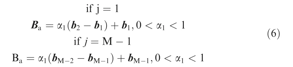
where α1is a ratio coefficient.After adding Ba,all control points can be re-ordered as follows.

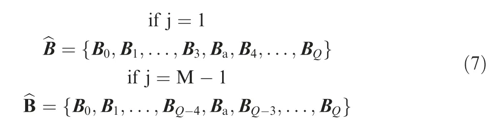
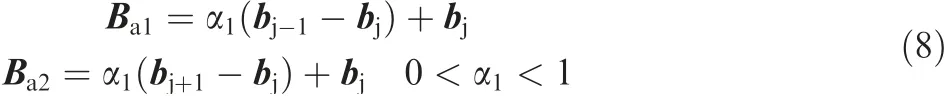
·Case II:if 1 ＜j ＜M-1,two control points are added.One, symbolized by Ba1, is added to the line segment bj-1bj,and the other,symbolized by Ba2,is symmetrically added to the line segment bjbj+1.

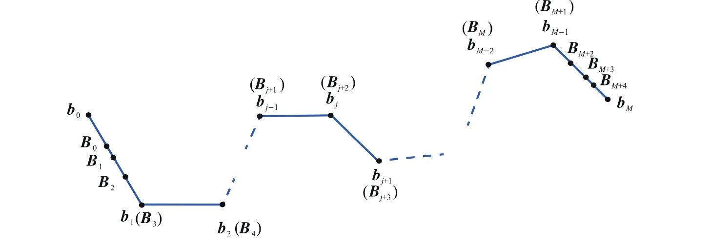
Fig.5 Initially selection of control points for the global method.

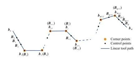
Fig.6 Control points during several iteration for the global method.

After adding Ba1and Ba2,all control points can be reordered as follows.

Based on the new series of control points,a new B-spline curve can be constructed.That is,adding new control point leads to the change of B-spline curve,and as a result,the value of εi,which is related to the corner point bj,will be changed correspondingly.Actually,it is aimed to reduce εito the acceptable level through this kind of means.In the case of critical condition,it is expected that the following equation holds.

Now,α1can be solved from Eq.(10).If 0 ＜α1＜1,it means that the new control point(s)can be added by using Eq.(6)or Eq.(8).Otherwise,it implies that the added control point(s) will be outside the line segment, i.e.b1b2,bM-2bM-1,bj-1bjor bjbj+1.In this case,α is artificially set to be 0.5 to ensure that the added control point(s)can be inside the corresponding line segment.For the convenience of expression,Q is updated as Q+1 and Q+2 for Case I and Case II,respectively.From Eq.(3),it can be observed that the knot vector is influenced by Q.As a result,once the control points are updated,the data of Q is correspondingly changed.In this case,the knot vector should be updated by Eq.(3).It should be pointed out that setting α1=0.5 cannot ensure εi≤εw,and a further optimization,which is described below,is still desired.

2.2.2.Global optimization of the tool path

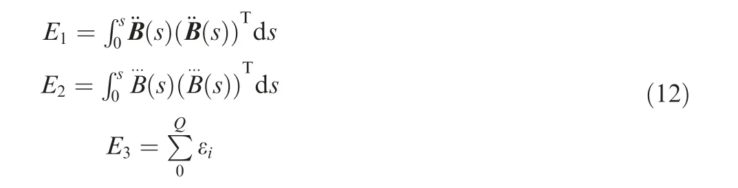
The above method only smoothes some certain corners,and a global optimization,which is expected to ensure the good smoothness and tolerance of final curve,is detailed as follows.Note that the series of the control points updated from Section 2.2.1 are the initial control points group Bi(i=0,4,5...,Q)used in this section.The objective function is expressed as follows by adding an error condition item into Eq.(24)corresponding to the local smoothing method.

with

where β and γ are the weighted coefficients.Iterative algorithm for global optimization is detailed as follows.

(1)If the maximum error appears at the ith control point,its error can be symbolized as εiaccording to the definition in Eq.(5).If εi＞εw,go to Step(2),otherwise,stop the iteration.

(2)The errors related to the two adjacent control points of the ith control point,i.e.εi-1and εi+1,are calculated and compared.If εi-1＜εi+1,add a new control point to the line segment BiBi+1,otherwise,add a new control point to the line segment Bi-1Bi.For the convenience of study,the new control point is treated as being added to line Be1Be2with e1=i+g and e2=i+g+1.If εi-1＜εi+1,g=0,else g=-1.Note that if i=4,the maximum error occurs at first corner,and in this case g=0,while if i=Q-3,the maximum error occurs at last corner,and correspondingly,g=-1.

(3)The added control point can be calculated as follows.

After adding Ba,all control points can be grouped as follows.

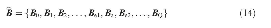
(4)Substitute α2into Eqs.(13)and(14)to generate the new control points. Update the control points Bi(i=0,1,2...,Q)with^B,and go to Step(1).

Finally,a global smoothing curve can be obtained only if the maximum error of the modified curve respect the tolerance.

2.3.Local corner smoothing method

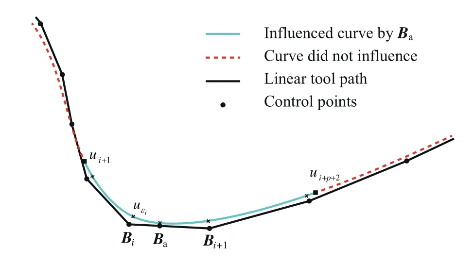
Fig.7 Local support characteristic of B-spline.

In this section,a local optimization method is proposed to smooth the tool path with corners.After local smoothing,the kth local corner will be consisted of a curve and two line segments,and the G3 continuity should be satisfied at the two junction points between the curve and the lines.In this section,a symmetric quintic B-spline curve with 7 control points is built,shown as Fig.3.The knot vector U=[00 0 0 00 0.5 1 11 1 1 1]is used to generate the B-spline curve.Corresponding to this case,the start and the end points of the generated curve will coincide with the first and the end control points of the curve,respectively.The G3 continuity at the junction points can be expressed as follows.16

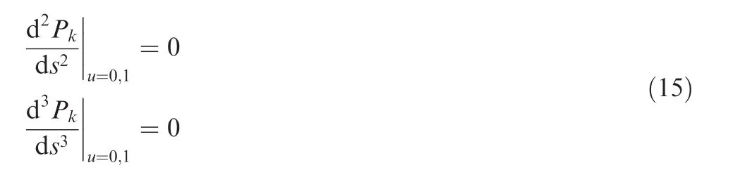
It can be proved that for any dk,1,dk,2and dk,3with the condition of dk,1≠0,Eq.(15)is satisfied,as can be seen in Appendix B.

The smoothed curve of the local tool path is constrained by

where the εwis the desired tolerance of tool tip position.The control points can be calculated by

Because of the symmetry,the distance between Pk,5and Pk,6equals dk,1.The distance between Pk,4and Pk,5equals dk,2,and the distance between Pk,3and Pk,4equals dk,3.Then,the control points can be remarked asdisplaystyle

F(xk)is a function with variables dk,1,dk,2and dk,3,and xk=[dk,1dk,2dk,3].

To obtain the smoothed curve,the values of dk,1,dk,2and dk,3should be determined first.According to Eq.(16),the following equation can be obtained.

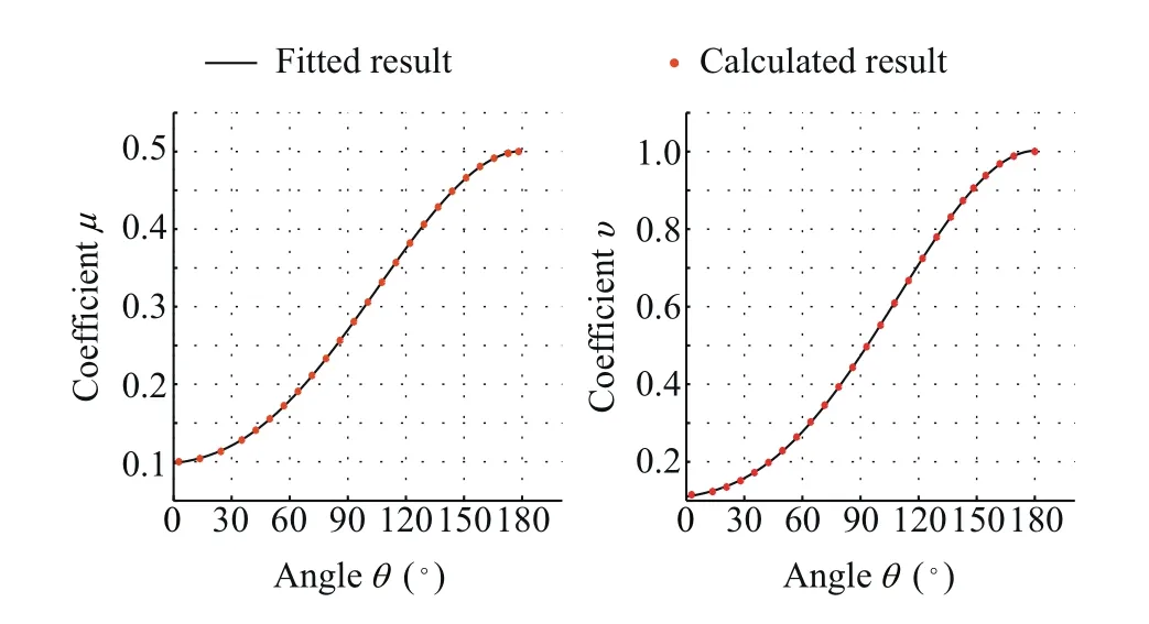
Fig.8 Calculated and fitted results for the ratio coefficients of μk and νk.

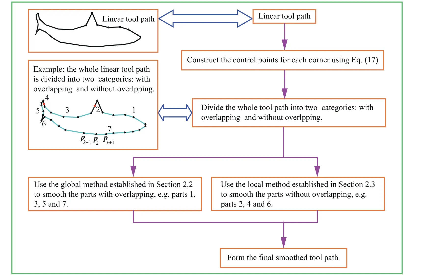
Fig.9 Smoothing procedure of the whole tool path.

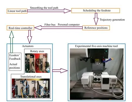
Fig.10 Experimental procedure on an open experimental five-axis machine tool.

The Eq.(20)can be written as a matrix

with

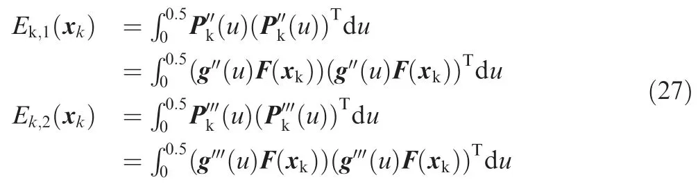
It is known that the derivation of position vector with respect to the curve length greatly influences the kinematics performance,and small acceleration and jerk can result in a better kinematics performance.The strain energy Ek,124and the jerk energy Ek,225can be expressed as follows.

where skis the total arc length of curve Pk.Ek,1(xk)is directly related to curvature of tool path,while Ek,2(xk)is implicitly associated with the fluctuation of the curvature.It should be pointed out that good smoothness of a curvilinear tool path,which is usually characterized by small curvature peak together with the small curvature fluctuation,can ensure steady motions of the axes.Based on this understanding,small values of Ek,1(xk)and Ek,2(xk)can lead to good kinematics performance.

To obtain a good kinematics performance,the following objective function is derived.

Fig.11 Comparison of the curvatures obtained by the proposed local method and the local method in Ref.16.

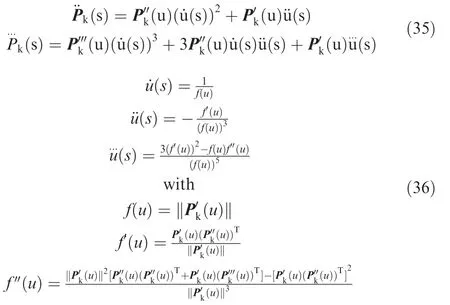
where βkis a ratio used to balance Ek,1and Ek,2.Minimizing the objective function gives a curve with better kinematics performance.From Eqs.(35)and(36),it can be found thatandare complex fractions of parameter u,and thus,Ek,1and Ek,2are actually difficult to be calculated.To simplify Eq.(24),andare replaced byandrespectively.Because a quintic quasi-uniform B-spline curve and seven control points are selected,the whole curve can be divide into two symmetric parts,i.e.u ∈[0,0.5]and u ∈(0.5,1],and each part can be described by an analytical function.Because of this symmetry,it is actually only needed to calculate the value of Ekwhen u ∈[0,0.5].Corresponding to this interval,the curve can be described as

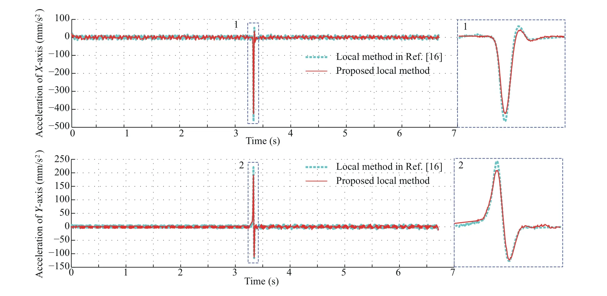
Fig.12 Comparison of acceleration for the corner with the angle being 30°.

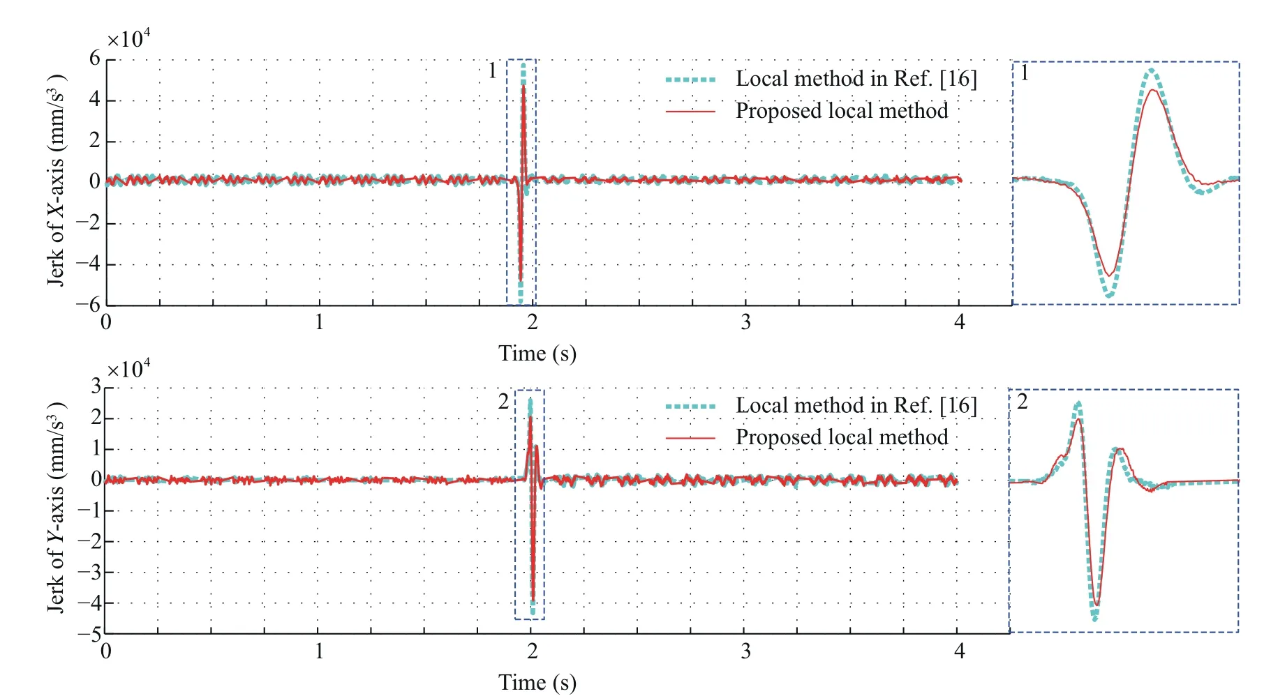
Fig.13 Comparison of jerk for the corner with the angle being 45°.

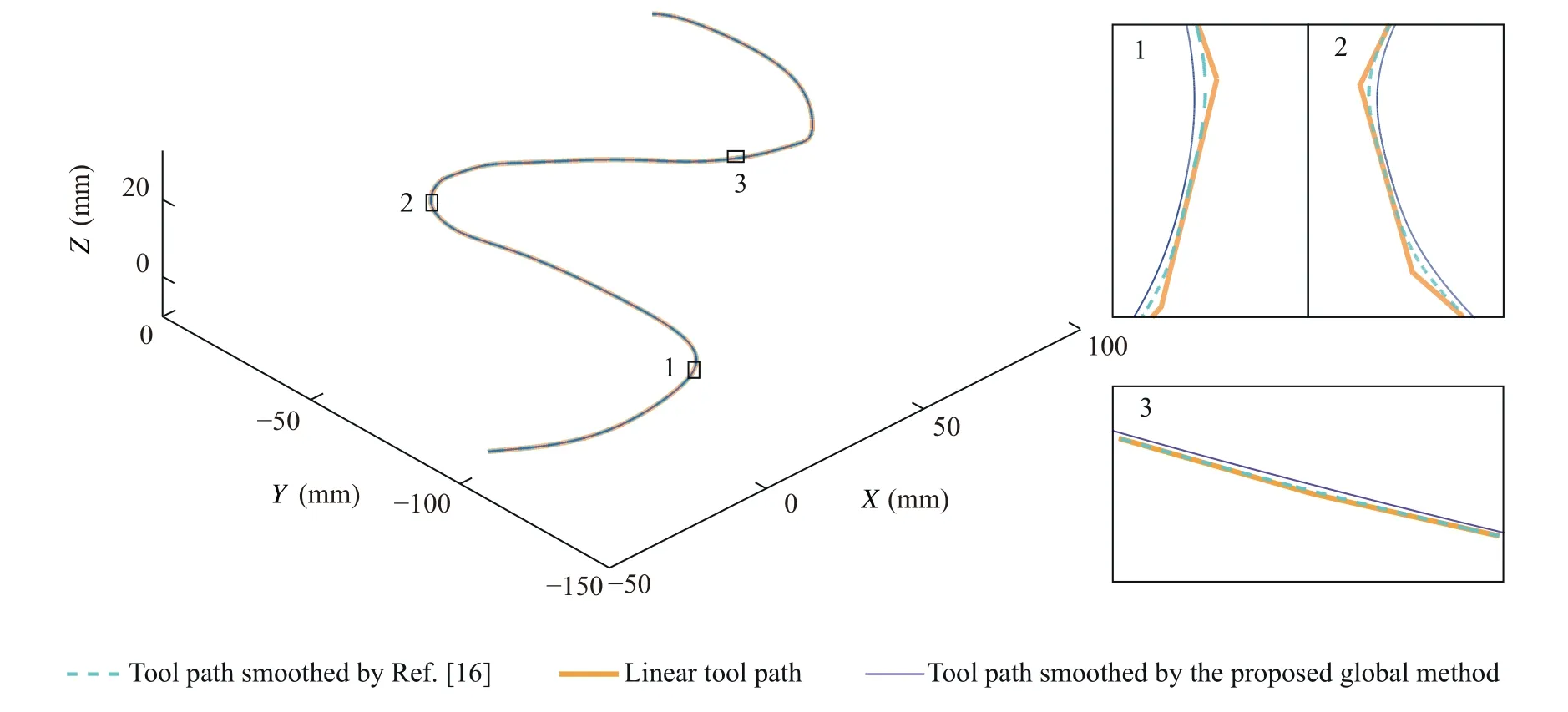
Fig.14 Smoothed 3D trajectory.

With the aid of Eq.(25),the following equation can be easily calculated.

with

The objective function is

Based on the above derivations,how to analytically select dk,1,dk,2and dk,3will be studied below.Focus is put on how to establish the relationship between the corner angle θ and the distances,i.e.dk,1,dk,2and dk,3.Without the loss of generality,illustration on constructing B-spline will be made on the kth local corner with the angle being θ and the three corresponding tool tip position points being pk-1,pkand pk+1.Because of the geometric invariance,the shape of B-spline curve is independent of the coordinate system.For the convenience of illustration,the origin of the local coordinate is selected as pk-1,and the X-axis is aligned with line pk-1pk.Thus,the coordinates of the pk-1,pkand pk+1can be expressed as follows.θ is the corner angle varying from 0 to π.Note that to avoid the overlapping phenomenon shown in Fig.2,lis length of the corner's line segments,which are selected to have relatively large value.Once the corner angle θ is given,the values of dk,1,dk,2and dk,3can be solved from Eq.(28).After setting μ=dk,1/dk,3and ν=dk,2/dk,3,triangle functions can be used to fit μ and ν follows.

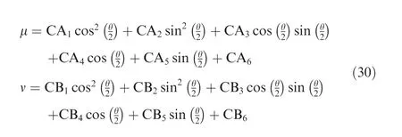
where CAκand CBκ(κ=1,2,...,6)are the fitting coefficients.Fig.8 illustratively shows the fitted relationship between θ and the ratios μ and ν.It is importantly commented that Fig.8,which explicitly shows the values of μkand νkcorresponding to each corner angle θkrather than iteratively solving Eq.(28),can be directly used to calculate Eqs.(2)and(17)involving the values of μkand νk.The details are shown below.

(1)Find the values of μkand νkfrom Fig.8 for a given θk.

(2)Solve dk,3directly based on Eq.(21)and the values of μkand νkobtained from Step(1).

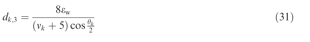
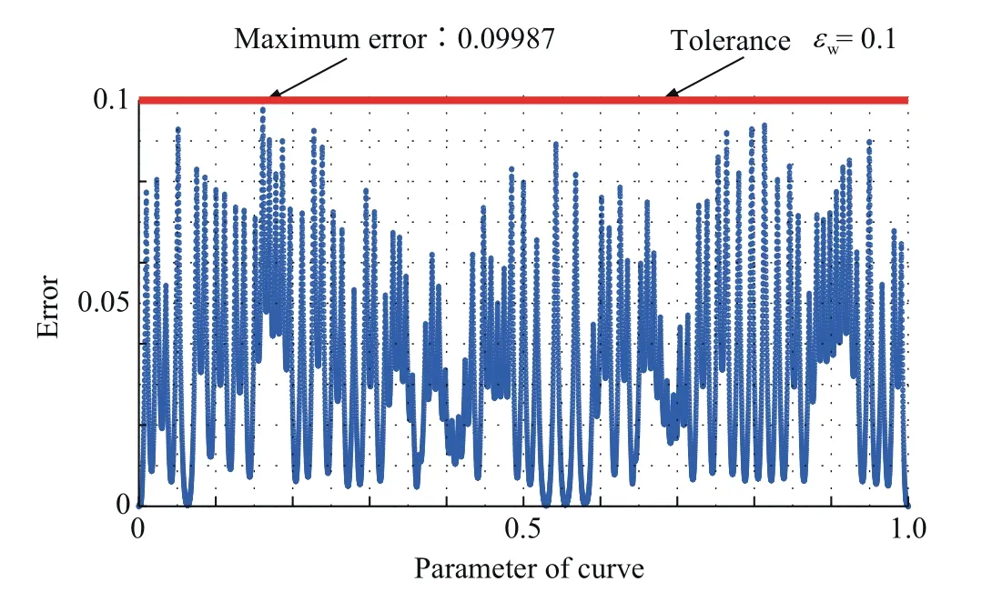
Fig.15 Error between smoothed and linear 3D trajectory.

(3)Solve dk,1,dk,2by dk,1=μkdk,3and dk,2=νkdk,3.

Finally,substituting the obtained dk,1,dk,2and dk,3into Eq.(17)gives the control points,which are used to construct the local B-spline curve corresponding to the kth corner.

2.4.Smoothing procedure of the whole tool path

Section 2.2 describes the method on smoothing the corners with overlapping,while Section 2.3 describes how to construct a local B-spline curve corresponding to a certain corner without overlapping.In this section,a procedure on smoothing a tool path,which involves some parts with overlapping and some parts without overlapping,will be given.The whole application flowchart is shown in Fig.9.

(1)For the tool path with the tool tip position points being pk(k=0,1,2,...,N),construct the control points Pk,fcorresponding to the kth corner by using Eq.(17).

(2)Divide the whole tool path into two categories with overlapping effects and without overlapping effects according to Eq.(1),as described in Section 2.1.

(3)Smooth the parts with overlapping by using the method described in Section 2.2.

(4)Smooth the parts without overlapping by using the method described in Section 2.3.

(5)Connect the results obtained from Steps(3)and(4)to form the finally smoothed tool path.

3.Simulation and experimental verification

The machine tool adopted in our previous work26is utilized to verify the proposed method.The machine is an open five-axis machine,which is built based on a three-axis machine tools with a rotary table.The experimental procedure is shown in Fig.10.First,the linear tool path is smoothed by proposed method. Next, feedrate planning is conducted for the smoothed tool path.Then,based on the planned federate,the reference positions of the tool path are generated,which can also be considered to compensate the influences of machine tools'geometric errors by adopting the method proposed in Refs.27-29.The friction characteristics are identified by using the methods established by Huang et al.30,31,which fully take the electromechanical characteristics of servo drives into consideration.Finally,online machining is conducted through the computer and real-time controller.Two kinds of comparisons are design to verify the advantages of the proposed methods.One uses the same feedrate planning to compare the acceleration and jerk,while the other uses the jerk limit method with same limitation to plan the feedrate and then compares the machining time.

3.1.Verification of local smoothing method

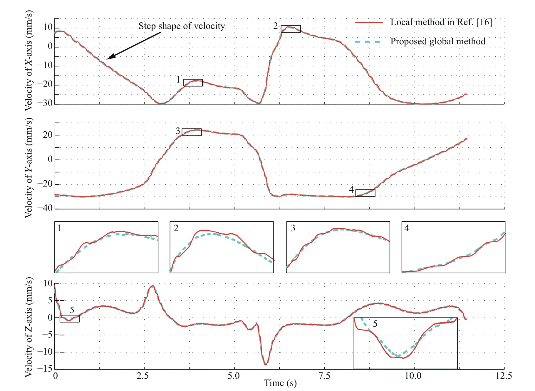
Fig.16 Comparison of the velocity corresponding to the 3D tool path in Fig.14.

A series of corners with different angle are used to show the advantages of the local corner smoothing method.The tolerance is given as εw=0.1 mm.The smoothed tool path can be obtained by the proposed local smoothing method.Fig.11 shows the comparison of the curvatures obtained by the proposed method and the results by using the method reported in Ref.16.It can be easily observed that the proposed method can lead to a lower curvature peak.Especially,the proposed method shows more excellent processing effect for sharp corners,as shown in Fig.11(a)-(c).It is also noticed that as θ is close to π,the generated curvatures obtained by the proposed method are almost the same as those reported in 16.

To conveniently compare the acceleration and jerk,the same feedrate is used for the proposed local smoothing method and the local corner smoothing method reported in Ref.16.The feedrates are set as 3 mm/s and 5 mm/s for the corners with the angles being 30°and 45°.Fig.12 compares the acceleration for corner with the angle being 30°at the feedrate of 3 mm/s.It can be easily observed that the proposed method corresponds to a lower acceleration.At the same time,compared with the method in Ref.16,the acceleration peak values of the proposed local corner smoothing method can be reduced by 9.03%and 13.37%for the X-and Y-axes,respectively.Fig.13 gives the jerk comparison for the corner with the angle being 45°at feedrate of 5 mm/s.The jerk peak value can be reduced by 17.23% and 10.56% for the X- and Y- axes,respectively.

3.2.Verification of global smoothing method

In this section,a 3D and a 2D tool paths are employed in simulation and experiment to verify advantages of the proposed global corner smoothing method.The tolerance is given as εw=0.1 mm.The 3D trajectory is shown in Fig.14.The heavy,dot and fine line mean the tool path without smoothing,smoothed by Tulsyan and Altintas'method and smoothed by the proposed global method,respectively.Fig.15 shows the error between smoothed and linear 3D trajectory,and it is within the prescribed tolerance.

A fixed velocity of 30 mm/s is used in experiment to guarantee the machine limitations,i.e.the jerk limitation,the acceleration limitation and the velocity limitation.The parameter interpolated by minimal feed fluctuation method is used to calculate the interpolation parameter.32Then,from experiments,the velocity, acceleration and the jerk are obtained and recorded.Fig.16 shows the comparison of velocity.It can be easily observed that the proposed global method has a more smoothed velocity.

During the experiment,the feedrate is fixed.Therefore,the following equation can explain why the global smoothing method has a smooth velocity and small fluctuation of acceleration and jerk.

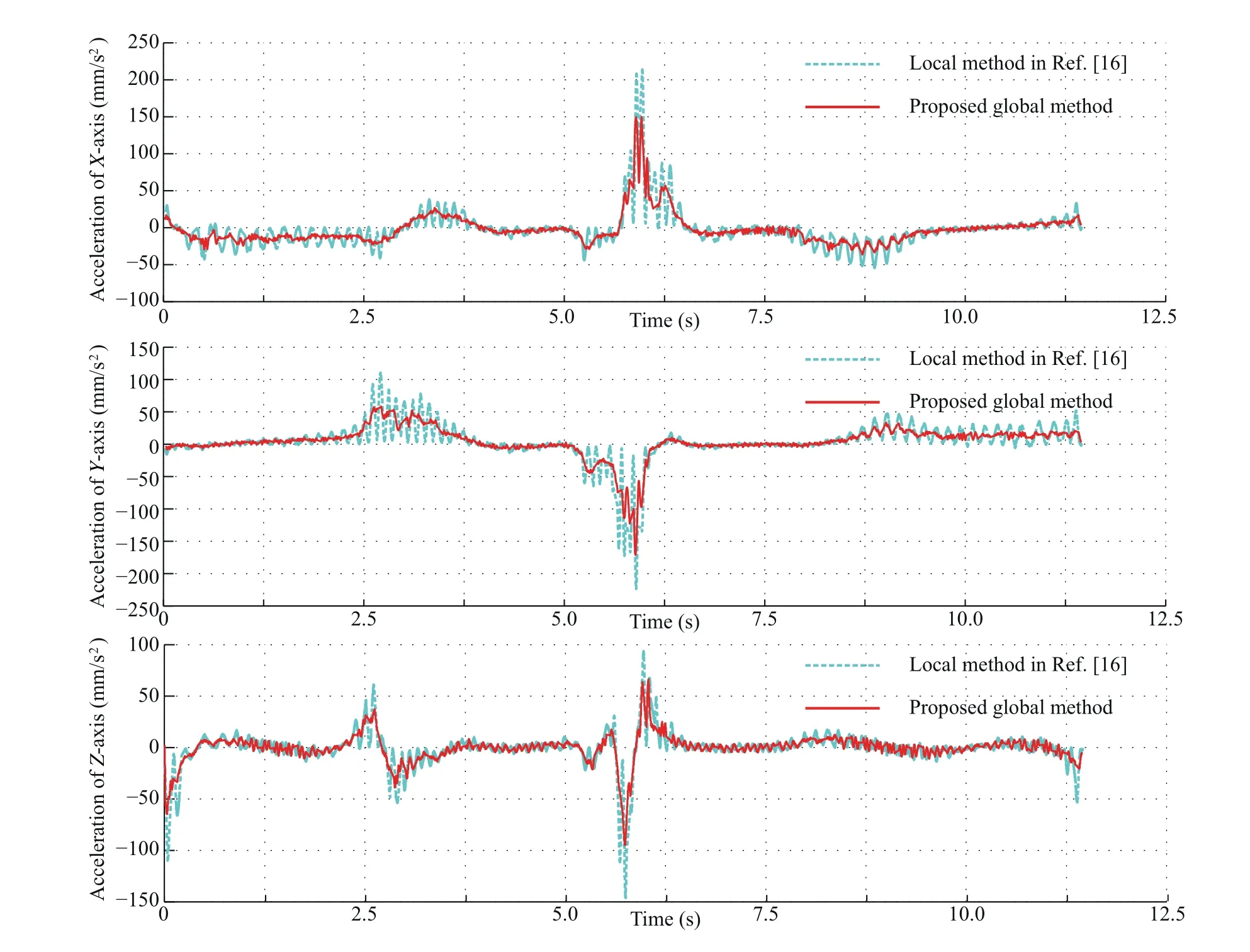
Fig.17 Comparison of the acceleration corresponding to the 3D tool path in Fig.14.

Fig.18 Comparison of the jerk corresponding to the 3D tool path in Fig.14.

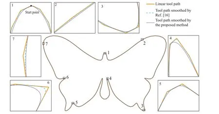
Fig.19 The smoothed 2D butterfly trajectory.

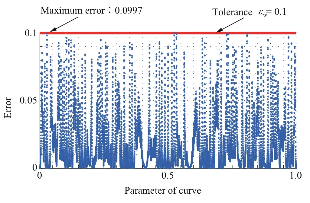
Fig. 20 Error between smoothed and linear 2D butterfly trajectory.

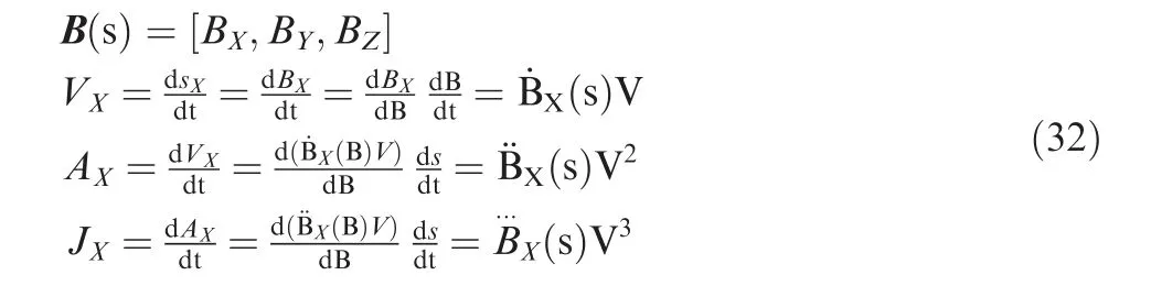
where B(s)is the expression of the smoothed curve.BX,BYand BZare the position coordinates of the smoothed curve relative to each axis.V is the fixed feedrate during machining.This equation takes X-axis as an example for illustration,and VX,AXand JXare the velocity,acceleration and jerk related to X-axis,respectively.Note that local method smoothes the linear segment by inserting a micro-Spline at each corner,and as a result,the corner is consisted of line,spline and line.For the tool path smoothed by the local method,the junctions between the smoothed curve and linear tool path have constant value ofThe values ofandare zeros.Thus,the velocity changes when machining the part with splines,while it keeps a constant when machining the line part.This phenomenon will result in a step shape of velocity,as observed in Fig.16.The acceleration and jerk will have a wave from zero to the peak value,and then return to zero.However,the global method proposed in this study takes several corners as the whole part.As a result,the velocity changes smoothly.The acceleration and jerk will also change with less fluctuations,as shown in Figs.17 and 18.Fig.17 compares the acceleration.It can be observed that the global method greatly reduces the value and fluctuation of acceleration.The peak values of accelerations related to X-,Y-and Z-axes can be reduced about 29.9%,23.42% and 35.04%, respectively.Fig.18 gives the comparison of jerk.It can be seen that the peak values of the jerks associated with X-,Y-and Z-axes can be reduced by 43.72%,42.95%and 56.58%,respectively.

The 2D butterfly curve is also smoothed by the proposed method,as seen in Fig.19.Fig.20 shows the error between smoothed and linear 2D tool path,and it is also within the prescribed tolerance.

A jerk limited acceleration profile is used to generate the feedrate scheme,10and the minimal feed fluctuation method is used to calculate the corresponding parameter.The feedrate acceleration and jerk limits are set as F=50 mm/s,Amax=150 mm/s2and Jmax=2000 mm/s3,respectively. The interpolation period is set as Ts=5×10-4s.Fig.21 shows the comparison of machining speed.It can be easily observed that the proposed global method has a higher efficiency than the G3 local smoothing method.The time consume reduced by 8.38%.

4.Conclusion

The tool path,which is consisted of linear segments,has discontinuity on geometry,and will thus result in the discontinuity on motion.Because of this,smoothing tool path is needed.In this paper,a global method together with an improved local method is proposed to smooth the tool path consisting of linear segments by using a quinic quasi-uniform B-spline to approach the linear tool path.The local corner smoothing method is carried out by minimizing an objective function consisting of strain energy and jerk energy of curve.Especially,a relationship between the corner angle and the ratio of control points of smoothed curve is explicitly established to facilitate directly finding the ratio of control points for a known corner.Simulation shows that the proposed local smoothing method can result in a lower peak value of the smoothed curve,and experiments show that the proposed local smoothing method leads to a lower acceleration when machining.The global corner smoothing method proposes an objective function,which is related to strain energy,jerk energy and errors between generated curve and linear tool path,to generate the globally smoothed tool path,which can satisfy the G3 continuity.The global method realizes smoothing the tool path in an error-controllable way. Experiments on an open five-axis machine show that the proposed global corner smoothing method is more efficient,and can produce a lower acceleration and jerk fluctuation in machining.

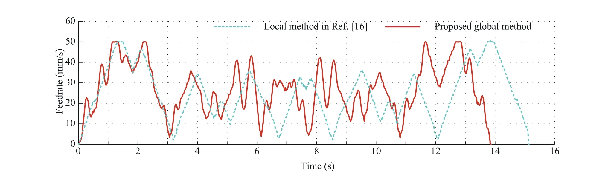
Fig.21 Comparison of the velocity corresponding to the butterfly tool path in Fig.19.

Acknowledgements

This research has been supported by the National Natural Science Foundation of China under Grant Nos.51675440 and 11620101002,National Key Research and Development Program of China under Grant No.2017YFB1102800,and the Fundamental Research Funds for the Central Universities under Grant No.3102018gxc025.

Appendix A.Brief introduction of B-spline curve

The B-spline curve B(u) is defined by control points Bi(i=0,1,2,...,n),basis function Ni,pand curve degree p.16

The basis functions Ni,pare defined by the knot vector U=[u0,u1,...,un+p+1]and geometric parameter u,as follows

where the first subscript i is the serial number of basis function,while the last subscript p is the degree of basis function.

Appendix B.Proof of Eq.(15)

By referring to Ref.16,the following derivations are achieved.

The derivation of Pkwith respect to u with u=0 can be expressed as follows

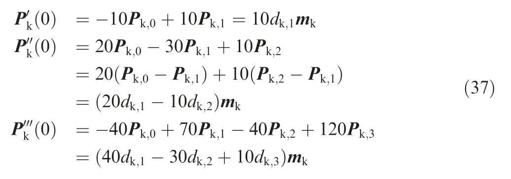
Substituting u=0 into Eq.(36),the following expression can be obtained.

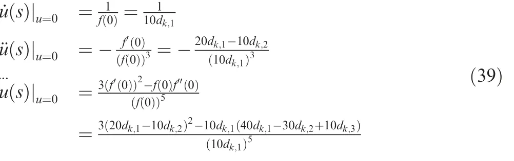
Combining Eqs.(38)and(39)with Eq.(35)gives

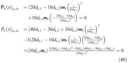
Following the similar procedure,it can be proved thatand