WANG Tao, YANG Kai-lin, GUO Xing-lei, XIE Sheng-zong, FU Hui, GUO Yong-xin

State Key Laboratory of Simulation and Regulation of Water Cycle in River Basin, China Institute of Water Resources and Hydropower Research, Beijing 100038, China, E-mail: taozyy@yahoo.com.cn

(Received November 30, 2011, Revised June 26, 2012)

EXPERIMENTAL STUDY HYDRAULIC ROUGHNESS FOR KAN TIN MAIN DRAINAGE CHANNEI IN HONG KONG*

WANG Tao, YANG Kai-lin, GUO Xing-lei, XIE Sheng-zong, FU Hui, GUO Yong-xin

State Key Laboratory of Simulation and Regulation of Water Cycle in River Basin, China Institute of Water Resources and Hydropower Research, Beijing 100038, China, E-mail: taozyy@yahoo.com.cn

(Received November 30, 2011, Revised June 26, 2012)

The Kam Tin Main Drainage Channel (KTMDC) is an important river for the city drainage in Hong Kong. The roughness and its variations have an obvious effect on the flood control capacity and the flow capacity. So physical model tests are designed to study the KTMDC. Due to its complex channel structure, the tests are completed in two steps. In Step 1, the energy loss is measured along the main channel without inflows, with all inflows and outflows being sealed. In Step 2, all the inflow and outflow structures are measured, with the sealed inflows and outflows being opened on the basis of Step 1. In each step, two schemes are employed. One of the key issues is the choice of suitable materials to make the model?s roughness similar to that of the prototype. According to the gravity similarity criterion, the 1:25 scale model is built, with the main channel made of Perspex. The facing slopes of the grasscrete and the stone masonry need to be roughened. A kind of the nylon net is selected to simulate the roughness of the stone masonry and the plastic lawn for the grasscrete facing slope. For the different structure reaches, the roughness coefficients are estimated based on the hydraulic theory. The rationality of the test results is verified in this study. The results of testing can provide a reliable basis for the renovation, the expansion, the optimization of this channel.

roughness, hydraulic character, channel, facing slope, grasscrete, masonry

Introduction

The Kam Tin Main Drainage Channel (KTMDC) is an important river for the city drainage in Hong Kong. A physical model is built for simulating the reach of the KTMDC between CHA 17+00 and CHA 25+50, as shown in Fig.1. Within this reach are two vehicular bridges (VB2 and VB4), one tributary branch channels (Tributary Channel B), three drainage inlets (Drain Pipe 4 and 5 (D4 and D5), Box Culvert 6 (BC6)) and a drainage outflow (Drain Pipe 7 (D7)). The channel cross-section is trapezoidal with a rectangular section in the middle and with transitions between the two forms of channel either end. The side slope of the channel is 1 vertical to 2 horizontal, and its side wall is covered with grass-crete panels or stone masonry. The channel gradient upstream of 0.68% is hydraulically steep while the gradient downstream of CHA 19+00 of 0.26% is mild. Due to the complexity of the prototype channel and the uncertai-nty about the surface roughness of its component parts, a physical model of KTMDC is needed to reveal the flow features and the hydraulic issues concerned. Through testing with a physical model, a reliable scheme is designed for the channel optimization, the reconstruction and the expansion. One of the issues in the study, the roughness coefficient of the drainage channel, is studied by the physical model testing.

The roughness is caused by the friction resistance between the flow and the surface or the obstacle, and it affects the hydraulic characteristics of the current[1-3]. Even in the ecology study, the friction to the flow plays an important role[4-6]. In the field of the management of water resources[7]and the wastewater reclamation or reuse system[8], the friction resistance should be taken into account in the current movement. The friction resistance in an open channel with vegetations was much studied by physical experiments[9]. The friction resistance is also a subject for theoretical studies[10].

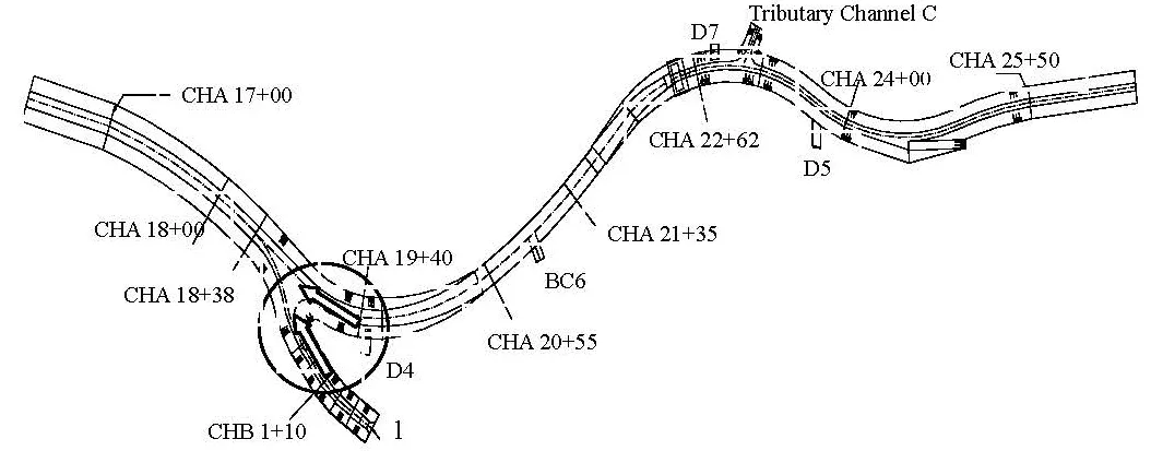
Fig.1 General layout of the drainage channel

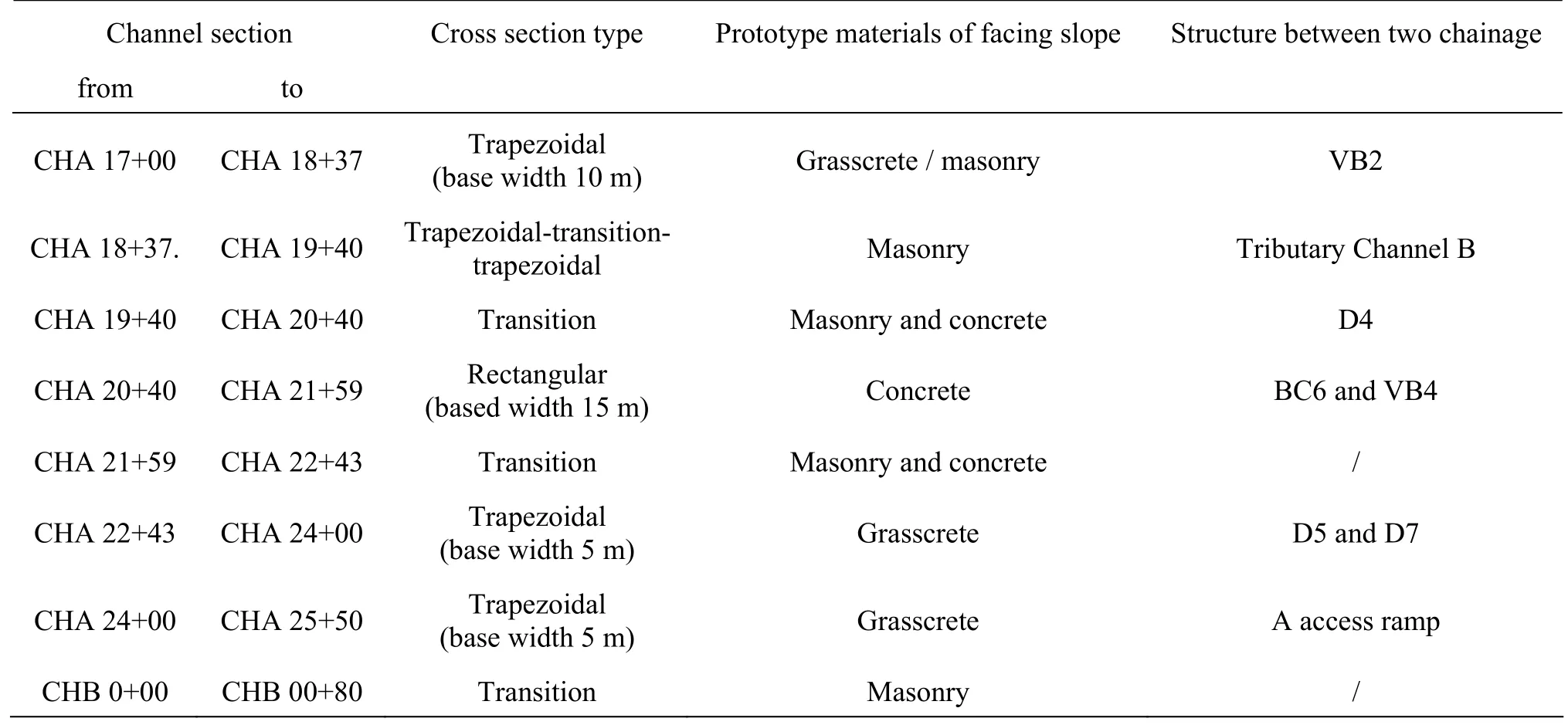
Table 1 Prototype conditions on different segments

The roughness is important for a river and a channel and affects their hydraulic characteristics seriously. Kalyanapu et al.[11]studied the effect of the land use-based surface roughness on the hydrologic model output. In their study, the model parameter sensitivity studies show that the runoff response is sensitive to the Manning roughness variations. Wang et al.[12]studied the effects of the roughness on the flow structure in a gravel-bed channel by using the particle image velocimetry. The experimental results show that the logarithmic-law region of the velocity profile changes with the size of the roughness elements. Chanson[13]studied the unsteady turbulence in Tidal Bores based on the effects of the bed roughness.

Although much research was carried out on the roughness for stream channels, there were few reports on the roughness for the densely vegetated surface and the complex section channel. Arcement and Schneider[14]suggested that the roughness value is determined by the factors that affect the roughness of channels and flood plains. In densely vegetated flood plains, the major roughness is caused by the grasses, trees, vines, and brush. The roughness of this type can be determined by measuring the vegetation density. Wang et al.[15]reviewed and analyzed the design criteria and the calculation methods of the roughness coefficients used for water transfer canals around the world based on the field investigation and the literature. They proposed approximate formulas for the roughness of the channels and correlative equations of the roughness. Shi et al.[16]studied the effect of vegetation submerged in the river on the roughness coefficients.

In this paper, the roughness coefficients are studied for different facing slopes of complicated channels.

1. Experimental setup

The roughness is an important issue in the design structure, the renovation, the expansion, and the optimization of a channel. This paper undertakes the physical tests of the roughness calibration. The studiedreach from CHA 17+00 to CHA 25+50 is in a shape of W-Type (as shown in Fig.1), with 7 types of crosssections, as listed in Table 1, and the Tributary Channel B flows into the main channel at Section CHA 18+38. The inflows to the D5, the BC6, the D4 and the outflow from D7 are arranged along this river segment, as shown Fig.1 and Table 1. The typical cross-section profiles for the trapezoidal channel and the rectangular channel are as shown in Fig.2. From Fig.2, the small drainage channel is designed in the channel base for draining the low flow in the nonflood season.

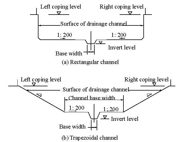
Fig.2 Typical cross-section profile for trapezoidal channel/ rectangular channel

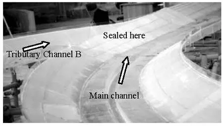
Fig.3 Sealed outlet of Tributary Channel B

The roughness calibration follows two steps. In Step 1, in order to measure the energy loss along the main channel without the bridges, the inflows from channel tributaries, the box culvert and the drainage pipes, all inflows and outflows are sealed, as shown Fig.3. The roughness coefficient so obtained would then represent predominately the effect of the boundary friction energy loss and the local energy loss along the main channel. In Step 1, the flow is only through the main channel, the test discharge obtained is 79 m3/s, 103 m3/s, 134 m3/s, respectively. In Step 2, the overall energy losses, including those from the main channel, the tributaries, all the inflow and outflow structures are measured. The sealed inflows and outflows are to be opened, as shown in Fig.4(a). Tributary Channel B is connected with the main channel, as shown Fig.4(b), whose location is denoted by a circle in Fig.1. VB2 is built in the segment from CHA 18+18 to CHA 18+27, where two bridge piers stand on the channel base to sustain the bridge deck, as shown in Fig.5. The two bridge piers provide some local resistance to the flow. The boundary condition and the pipe flow conditions in Step 2 are as shown in Table 2. In testing Step 1, the calibration is carried out first. With all boundary conditions and the model configurations similar to the prototype, the key parameters that need to be calibrated include the energy loss along the channel and the surface roughness coefficient which controls the over-all hydraulic performance and the flow capacity of the model, and they provide the basis for testing Step 2.

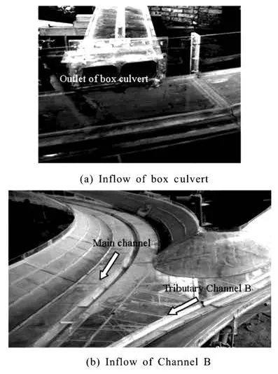
Fig.4 Open inflow connected with the main channel

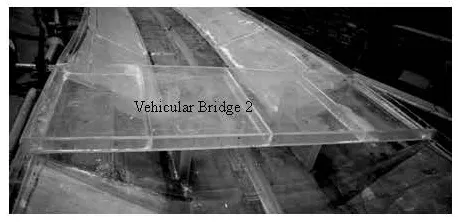
Fig.5 Vehicular Bridge 2

The design of the physical model of KTMDC is based on the hydraulic similarity theory. For free-surface flows, the hydraulic similarity criteria include the geometrical similarity and the gravity force similarity between the prototype and the model. The physicalmodels were built in a true undistorted scale of 1:25. The length of the reach of the KTMDC to be modeled is 850 m from CHA 17+00 to CHA 25+50. To ensure that the approach flows are representative of the prototype conditions as well as possible, subject to all scaling constraints, the models extend a sufficient dimension along each branch. The model extends to CHA 25+85 upstream and CHA 16+75 downstream. To replicate the flow and the boundary conditions as would be expected in the prototype, the roughness similarity is necessary. The roughness of the concrete is about 0.014, therefore, the roughness of the model material shall be 0.0082, close to that of Perspex. So the main channel is made of Perspex. In the bottle of the channel, the concrete is laid on all the facing bases. In the facing slope, the grasscrete, the masonry and the concrete are laid on different cross-sections, as shown in Table 1. Especially, the two schemes are designed to simulate the channel roughness in each step. The slopes of the grasscrete or the masonry, as shown in Table 1, are tested in the downstream from CHA 17+00 to CHA 18+38 as comparison schemes under the same boundary and flow conditions in each testing step, respectively. This means that the masonry facing slope is used in Scheme 1, and the grasscrete one in Scheme 2 from CHA 17+00 to CHA 18+ 38 when the testings in Step 1 and Step 2 are carried out, respectively.

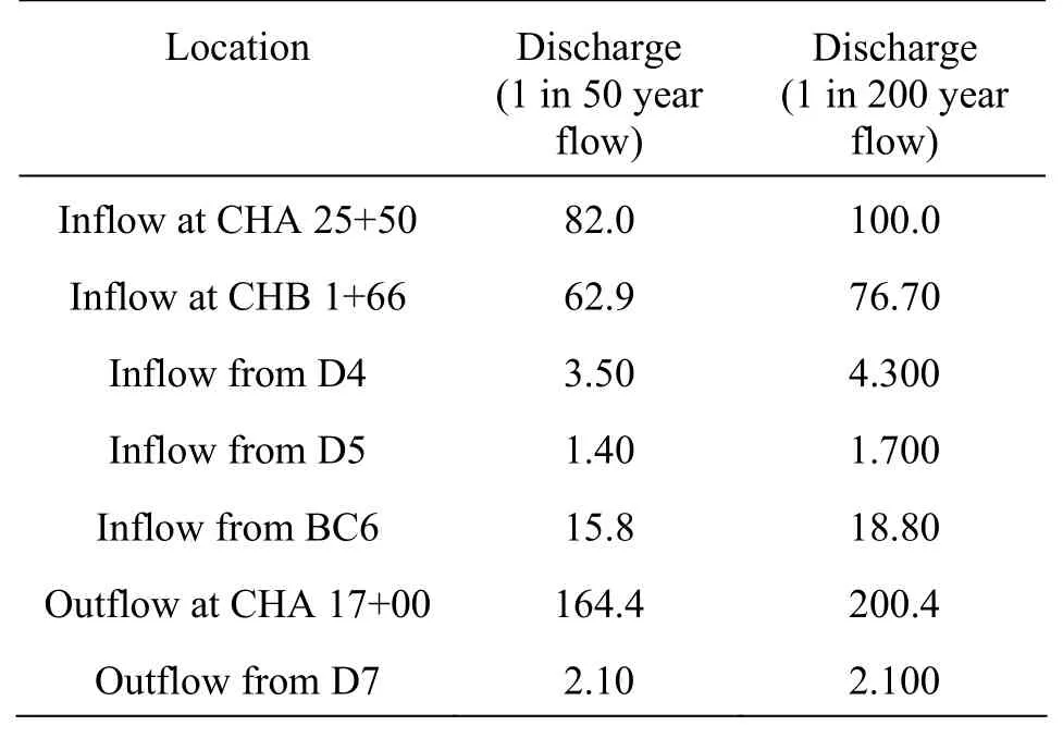
Table 2 Boundary conditions and pipe flow Conditions in Step 2 (m3/s)

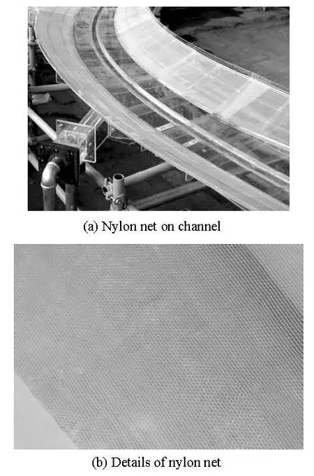
Fig.6 Nylon net simulating the stone masonry

The facing slopes of the grasscrete and the stone masonry need to be roughened. The roughness of the stone masonry is related with the size and the shape of the gravel particles. According to the information provided by the Project Provider, the theoretical roughness coefficient n of the masonry slope is around 0.021, which means that the roughness of the model material shall be 0.012. Several mesh materials are used to simulate the roughness of the stone masonry. According to the comparison of the many test results, a kind of nylon netting is shown to be suitable as a surface material to simulate the roughness of the stone masonry, as shown in Fig.6(a). The net is made of the nylon material, 0.0007 m thick. The holes of the net are of squares of 0.001×0.001 m2, as shown in Fig.6(b). The roughness of the grasscrete slope changes greatly with the vegetation conditions, the grass types, the growing season and others. Zhang et al.[17]shows that the hydraulic roughness of a turf used in the revetment ranges from 0.020 to 0.090, depending on different categories of soil, period of growth and way of reinforcement. Arcement and Schneider[14]classifies the roughness vegetation into four grades (as shown in Table 3) according to the vegetation conditions, that is, that of the small adjustment for values in the range of 0.002-0.01, that of the medium adjustment for values in the range of 0.01-0.025, that of the large adjustment for values in the range of 0.025-0.05 is large, and that of very large adjustment for values in the range of 0.05-0.1. According to the on-site assessment, the design requirements and the flow conditions, the roughness is found to be about 0.028, which requires that the roughness of the model material should be 0.016. In order to better simulate the natural characteristics of the grasscrete, the plastic lawns are laid on the grasscrete facing slope. Tests were carried out by changing the density of the plastic grass and the length and the width of the grass leaves for selecting a suitable grass, to keep the similarity with respect to the prototype grasscrete. A new plastic lawn is decided, as shown in Fig.7(a). The height of the grass is 0.016 m-0.021 m on the plastic lawn, as shown in Fig.7(b).The array of the grass is shown in Fig.8, in which each circle represents a cluster of grass and the black arrow shows the direction in which the grasscrete is laid, the same as that of the black arrow in Fig.7(a).

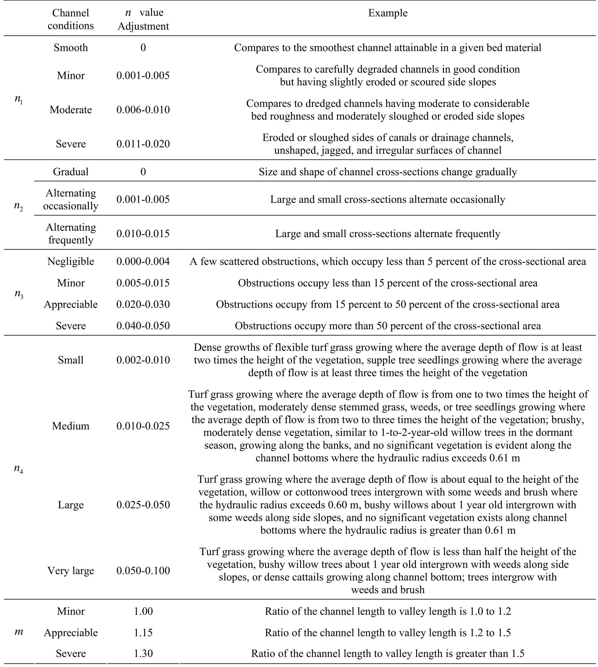
Table 3 Adjustment values for factors that affect the roughness of a channel[13]

The locations where the flow rate needs to be controlled and measured include CHA 25+50 (channel upstream), West Culvert, CHB 1+66 (Tributary Channel B), the SSS East Culvert, BC6, CHA 17+00 (channel downstream), D4, and D7. At each location a flow measurement equipment is installed to control the discharge. To examine the complex three-dimensional flow pattern along the KTMDC, Acoustic-Doppler Velocimetry (ADV) meters are used to measure the 3-D velocity to obtain the velocity distribution alone the channel. To measure the water levels, fixed and movable gauges are used. With the above experiment setup, the roughness calibration is carried out.

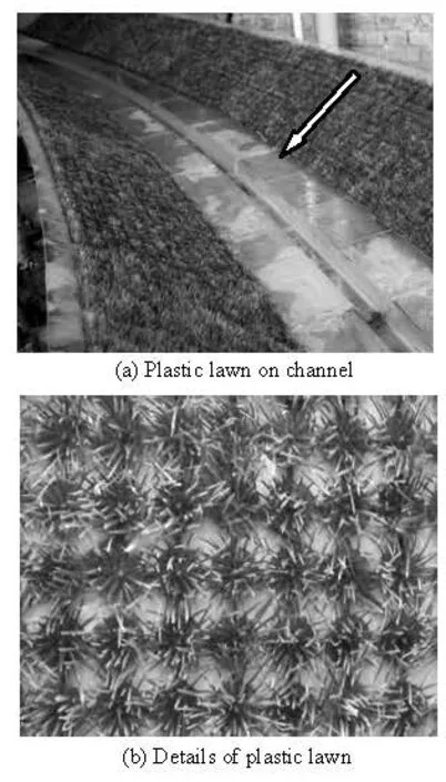
Fig.7 Plastic lawn simulating the grasscrete

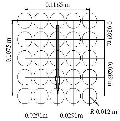
Fig.8 Array of plastic lawn

2. Roughness calibration and analysis

For natural rivers and artificial channels, the most important factors that affect the selection of the channel value n are as follows: (1) the type and the size of the materials used to cover the bed and the banks of the channel. (2) the shape of the channel. Cowan[14]developed a procedure for estimating the effects of these factors to determine the value ofn for a channel or a river. The value of n may be computed by

where nbis a base value of n for a straight, uniform, smooth channel in natural materials, n1is a correction factor for the effect of surface irregularities, n2is a value for variations in shape and size of the channel cross section, n3is a value for obstructions, n4is a value for vegetation and flow conditions,m is a correction factor for meandering of the channel. A stable channel is defined as a channel in which the bed is composed of firm soil, gravel, cobbles, boulders, or bedrock and the channel remains relatively unchanged throughout most of the range in the flow. For the base value of nb, the roughness of the concrete ranges from 0.011 to 0.018, and that of a firm soil from 0.020 to 0.032. The roughness of the rock cut is 0.025 for a smooth channel[13]. The values of n1, n2, n3and n4, are detailed in Table 3. Therefore, the hydraulic structure channel is very complex for the KTMDC where there are above five coefficients that affect the channel?s roughness. Because of the uncertain factors in Eq.(1) and Table 3, the roughness coefficients can not be calculated by Eq.(1), appropriately. But this equation provides a useful guidance for the experiment design and the roughness analysis.

There are three types of flow resistance in the open channel: (1) the friction resistance of the channel surface, (2) the local resistance, caused by sudden changes in the cross-section shape, (3) the energy dissipation in the turbulent flow. The above three flow resistances are governed by different resistance laws, and affect the flow characteristics and the roughness coefficients. The results of the tests are shown in Table 4 and Table 5 for Step 1 and Step 2. In Step 2, the conditions of the main channel, the Tributary Channel B and the pipe flow are as shown in Table 1. In the same step stage, the distinction between Test Scheme 1 and Test Scheme 2 is that in Test Scheme 1, the Masonry is used to cover the segment from CHA 18+38 to CHA 17+00, and in Test Scheme 2, the grasscrete is used. Comparing the test results, the conclusions are as follows.

The calibration of the roughness is conducted in steady state flow conditions under which the water levels and the velocities at the selected locations along the model channel are constant and can be measured. Manning?s roughness coefficient n is expressed in the steady non-uniform flow as follows

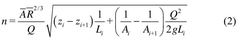
where n is the Manning?s roughness coefficient,A is the cross-section area, R is the hydraulic radius, Q is the flow rate, ziis the water level at the upstream cross-section (Section i), zi+1is the water level at the downstream cross-section (Section i+1),Liis the distance between the two cross-sections (from Section i to Section i+1). The values of the roughness coefficients in Tables 4 and 5 are explained as follows.

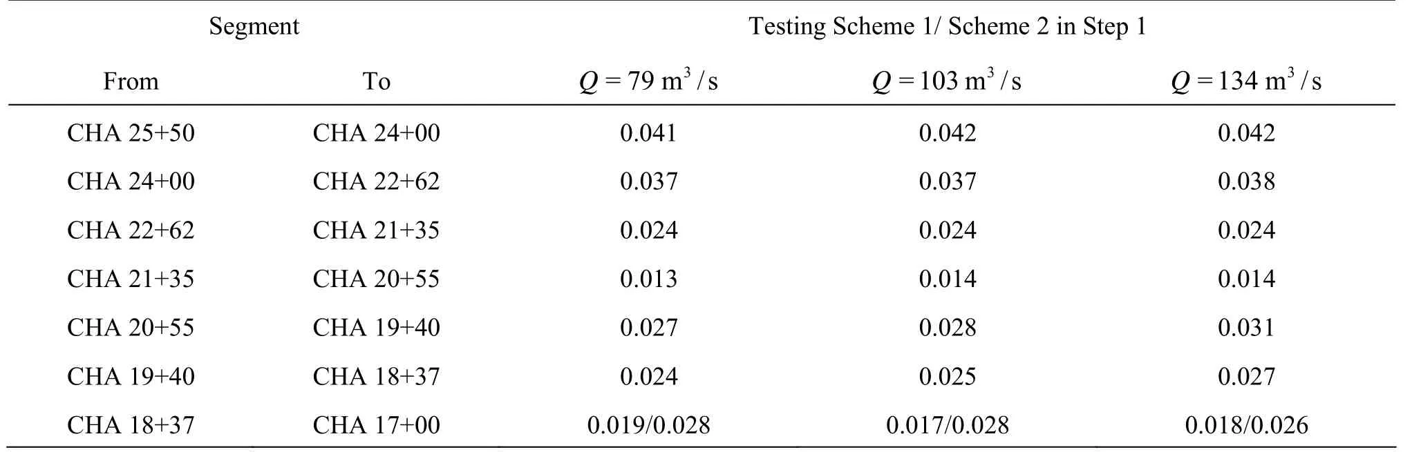
Table 4 Calibrated roughness comparisons in Step 1

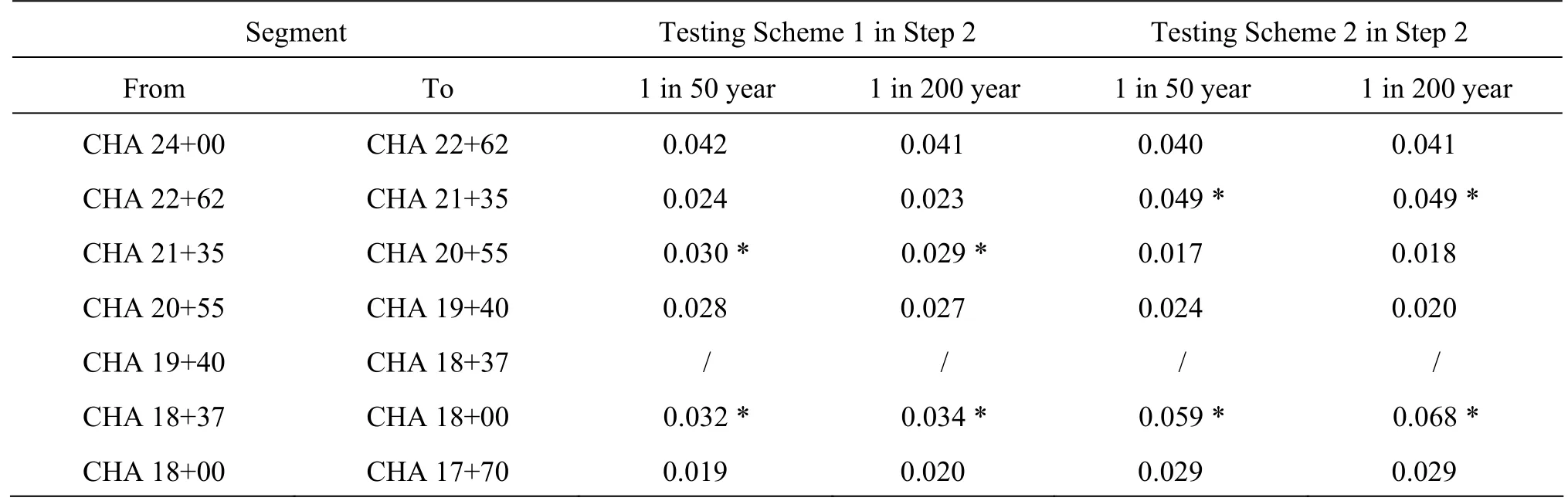
Table 5 Calibrated roughness comparisons in Step 2

At the upstream CHA 25+50-CHA 24+00, the model structure and the slope are not changed in Step 1 and Step 2. The roughness coefficient 0.041-0.042 is influenced by the turbulent flow caused by the access ramp built in this reach and the friction resistance of the channel surface. In the segment CHA 24+00-CHA 22+62, there are the inflow of D5 and the outflow of D7 for Step 2, and not for Step 1. The calibrated roughness coefficients are 0.037-0.038 (Table 4) for Step 1 and 0.040-0.042 (Table 5) for Step 2. The increasing Manning roughness is caused by the local flow mixing from the inflow and the outflow in Step 2. The segment CHA 22+62-CHA 21+35 is a transition, there is no inflow or outflow, but the hydraulic jump is observed near CHA 21+75 in the case of the flow that would occur once in 200 years in Step 2, which is why the Manning roughness changes from 0.023-0.024 to 0.049 (Tables 4 and 5). The additional energy loss by the turbulent flow is increased mainly by the hydraulic jump, not by the surface friction energy loss along the channel segment.

The middle segment (CHA 21+35-CHA 20+55) hasa uniform rectangular section. In Step 1, the energy loss is dominated by the surface friction of the main channel, so the Manning roughness coefficients are close to the value “n” of the concrete channel. Because of the inflow from BC6 in Step 2, the calibration roughness 0.017-0.018 (Table 5) in Step 2 is slightly higher than the value of 0.013-0.014 (Table 4) in Step 1. In the case of the flow that would occur once in 50 years in Step 2, a hydraulic jump is formed so it is not only the friction resistance of the channel surface that is measured, but also the turbulent mixing and the vortex head due to the energy dissipation in the hydraulic jump. So the measured roughness values of 0.030 and 0.029 (Table 5) are not simply the Manning roughness coefficients caused by the friction resistance of the surface material. In the segment from CHA 20+55 to CHA 19+40, the roughness coefficients are close in Step 1 and Step 2 stages because the hydraulic structure and the flow condition are changed slightly in this transition reach.

At the downstream (CHA19+40-CHA 18+38), Tributary Channel B is the inflow into the main channel. The confluence of two large streams induces strong impulse, mixing and dissipation. The originalManing?s formula, established on the bases of the single channel and the uniform flow, can not be applied, so the calibration Manning roughness is not done in Step 2. So their Manning roughness coefficients 0.024-0.027 (Table 4) are close to the value “n” of this meandering reach in Step 1.

At the downstream (CHA 18+38-CHA 18+00), the a bove mentioned three resistances, including the friction resistance of the channel surface, the local resistance caused by sudden changes in the crosssection shape, the local energy dissipation in the turbulent flow, exist due to the piers and the deck at VB2, located in the segment from CHA 18+18 to CHA 18+27. The local resistance coefficient depends on the shape of the structure in the flow and the surface friction resistance depends on the coefficient of roughness and the hydraulic radius of the channel section. In order to distinguish their interactions, a measurement point at CHA 18+00 is added in Step 2. Influenced by the local resistance of VB2, the roughness coefficients 0.032-0.034 for Scheme 1 and 0.068-0.059 for Scheme 2 (Table 5) are increased obviously in this segment. During testing under the case of the flow that would occur once in 200 years, the flow impacts on the duck of VB2 in Scheme 2. So a larger roughness coefficient 0.068 is obtained. The phenomenon does not occur under the case of the flow that would occur once in 50 years. Therefore, the roughness coefficients are deduced according to the three resistances in the segment. If one excludes the interference caused by the local resistance of VB2, the calculated Manning?s roughness of the segment from CHA 18+00 to CHA 17+00 is 0.019-0.020 and 0.029 (Table 5), which is close to the value of the calibration in Step 1. Thus, the test results are verified.

3. Conclusions

The calibration was carried out in two steps. In Step1, this calibration was done by measurement of the energy loss along segments of the channel initially without branch inflows so that energy losses were predominately due to the friction along the main channel. So the Manning roughness coefficient calibrated in Step 1 represents the basic hydraulic characteristics of the channel. This calibration is carried out for the main channel only to provide a basis for the comparison of the results obtained in testing Step 2. In Step 2, the inflow and outflow structures along the main channel, D4, D5, D7 and Tributary Channel B, are connected with the main channel. The bridges are added along the main channel. The overall energy losses including those from the main channel, the tributaries, all the inflows, outflow structures and the bridges are measured. The Manning roughness coefficients measured in Step 2 including the measured local resistances can be expected to vary with the discharge, the velocity or the flow pattern. So the calibrated roughness is more representative of the roughness of the existing channel. Its results can provide a reliable basis for the renovation, the expansion, the optimization of this channel.

The roughness calibration of the channel is a verycomplex task. In this study, some factors were not considered in the testing and analysis due to the limitations of the test condition, they should be taken into account in further tests.

Refernces

[1] WANG X. Y., YANG Q. Y. and LU W. Z. et al. Effects of bed load movement on mean flow characteristics in mobile gravel beds[J]. Water Resources Management, 2011, 25(9): 2781-2795.

[2] HUAI Wen-xin, HAN Jie and ZENG Yu-hong et al. Velocity distribution of flow with submerged flexible vegetations based on mixing-length approach[J]. Applied Mathematics and Mechanics (English Edition), 2009, 30(3): 343-351.

[3] FERRO V. Flow resistance in gravel-bed channels with large-scale roughness[J]. Earth Surface Processes and Landforms, 2003, 28(12): 1325-1339.

[4] HOOVER T. M., ACKERMAN J. D. and JOSEF D. A. Near-bed hydrodynamic measurements above boulders in shallow torrential streams: Implications for stream biota[J]. Journal of Environmental Engineering and Science, 2004, 3(5): 365-378.

[5]PENA E., ANTA J. and PUERTAS J. et al. Estimation of drag coefficient and settling velocity of the cockle cerastpderma edule using Particle Image Velocimetry (PIV)[J]. Journal of Coastal Research, 2008, 24(4, suppl.): 150-158.

[6] WU C. L., CHAU K. W. and HUANG J. S. Modelling coupled water and heat transport in a soil-mulch-plantatmosphere continuum (SMPAC) system[J]. Applied Mathematical Modelling, 2007, 31(2): 152-169.

[7]CHENG C. T., CHAU K. W. Flood control management system for reservoirs in China[J]. Environmental Modelling and Software, 2004, 19(2): 1141-1150.

[8]LU W. Z., LEUNG A. Y. T. A preliminary study on potential of developing shower/laundry wastewater reclamation and reuse system[J]. Environmental and Public Health Management, 2003, 52(9): 1451-1459.

[9]NENAL Laounia, YAN Zhong-min and XIA Ji-hong. Study of the flow through non-submerged vegetation[J]. Journal of Hydrodynamics, 2005, 17(4): 498- 502.

[10]YANG Sheng-fa, HU Jiang and LI Dan-xun et al. Some new data formulas for resistance flow in fluvial open channels[J]. Journal of Hydrodynamics, 2011, 23(4): 527-534.

[11] KALYANAPU A. J., BURIAN S. J. and MCPHERSON T. N. Effect of land use-based surface roughness on hydrologic model output[J]. Journal of Spatial Hydrology, 2009, 9(2): 51-71.

[12]WANG X. Y., SUN Y. and LU W. Z. et al. Experimental study of the effects of roughness on the flow structure in a gravel-bed channel using particle image velocimetry[J]. Journal of Hydrologic Engineering, 2011, (9): 710-716.

[13] CHANSON H. Unsteady turbulence in tidal bores: Effe-cts of bed roughness[J]. Journal of Waterway, Port, Coastal, and Ocean Engineering, 2010, 136(5): 247-265.

[14] ARCEMENT G. J., SCHNEIDER V. R. Guide for selecting Manning?s roughness. Coefficients for natural channels and flood plains[R]. United States Geological Survey Water-supply, Paper 2339, 1989.

[15] WANG Guang-qian, HUANG Yue-fei and WEI Jia-hua et al. Identification of roughness-coefficient value for the channel of the south-to-north water transfer(middle line) project[J]. South-to-North Water Transfers and Water Science and Technology, 2006, 4(1): 8-14(in Chinese).

[16] SHI Bing, WANG Chuan-yuan and YIN Ze-gao et al. Effect of vegetation submerged in river on the roughness coefficient[J]. Journal of Ocean University of China, 2009, 39(2): 295-298(in Chinese).

[17] ZHANG Wei, ZHONG Chun-xin and YING Han-hai. Experimental study on hydraulic roughness of revetment with grass cover[J]. Advances in Water Science, 2007, 18(4): 483-489(in Chinese).

10.1016/S1001-6058(11)60303-X

* Biography: WANG Tao (1975-), Female, Master, Senior Engineer