Stem taper functions for Betula platyphylla in the Daxing’an Mountains, northeast China
Muhammad Khurram Shahzad · Amna Hussain · Harold E. Burkhart · Fengri Li · Lichun Jiang
Abstract Accurate prediction of stem diameter is an important prerequisite of forest management. In this study, an appropriate stem taper function was developed for upper stem diameter estimation of white birch ( Betula platyphylla Sukaczev) in ten sub-regions of the Daxing’an Mountains, northeast China. Three commonly used taper functions were assessed using a diameter and height dataset comprising 1344 trees. A first-order continuous-time error structure accounted for the inherent autocorrelation. The segmented model of Max and Burkhart (For Sci 22:283–289, 1976. https ://doi.org/10.1093/fores tscie nce/22.3.283) and the variable exponent taper function of Kozak (For Chron 80:507–515, 2004. https ://doi.org/10.5558/tfc80 507-4) described the data accurately. Owing to its lower multicollinearity, the Max and Burkhart (1976) model is recommended for diameter estimation at specific heights along the stem for the ten sub-regions. After comparison, the Max and Burkhart (1976) model was refitted using nonlinear mixed-effects techniques. Mixed-effects models would be used only when additional upper stem diameter measurements are available for calibration. Differences in region-specific taper functions were indicated by the method of the non-linear extra sum of squares. Therefore, the particular taper function should be adjusted accordingly for each sub-region in the Daxing’an Mountains.
Keywords White birch · Taper function · Multicollinearity · Autocorrelation · Nonlinear regression
Introduction
White birch ( Betula platyphylla Sukaczev) is a valuable hardwood species of China and listed among the top ten species of the country. It covers an area of 10.38 × 10 6 (M) hectares, with a total volume of 1033 M m 3 (Xu et al. 2019). It has been registered as one of China’s science and technology research tree species. Stands of white birch are widely dispersed across the north and southwest. The largest area of this species with the largest stand volume lies in northeast China. This region contains abundant forest resources and is one of the most important areas of timber production. As per the latest National Forest Inventory (NFI-8), the northeast region has an area of 32.71 M ha under forest with 28,180 M m 3 standing volume (Zeng et al. 2015). The Daxing?an Mountains are located in Heilongjiang province and in the eastern part of Inner Mongolia, and white birch is the second major tree species in this area, the major species is Dahurian larch ( Larix gmelinii Rupr.). The standing volume of white birch is distributed over 1.9 M ha and is 128 M m 3 , which is 25% of the total standing volume of tree species of the region (Samuelsson 2006).
White birch possesses excellent properties in terms of growth rate, adaptability, wood texture, structure, and durability. Additionally, it is the primary source for pulp in papermaking, for plywood and for furniture (Xu et al. 2016). Its commercial and economic uses extend globally, for example, Chinese white birch plywood is the principal item of wood imports into the USA. The wood contains exceptional physical characteristics that allow for natural and dyed finishes, cabinetry, and lamination (Far-East-American 2012). With the importance of white birch, a stem taper equation would be beneficial for sustainable management of the species. Stem taper functions have been recommended as an effective tool based on several studies to predict stem diameter ( d) at any height as well as to estimate merchantable and total volumes (Rojo et al. 2005; Trincado and Burkhart 2006; Li and Weiskittel 2010; ?zcelik et al. 2011). The majority of such functions require total tree height ( H), diameter at breast height ( D), and height ( h) of d above the ground as independent variables (Berhe and Arnoldsson 2008; Hjelm 2013). Stem taper functions supersede the customary stem volume models as they estimate d, merchantable height to any diameter above the ground, the volume of a log of any length and at any height from the ground, in addition to merchantable and total stem volume (Kozak 2004).
Stem taper equations may be divided into three categories: simple polynomial, segmented polynomial, and variable-exponent equations. Simple taper equations describe the changes from base to crown tip in diameter by a single function (Behre 1923; Matte 1949; Osumi 1959; Kozak et al. 1969; Demaerschalk 1972). Simple fitting and easy integration to calculate volume are characteristic features of these functions. Such functions adequately account for the middle stem portion but are significantly biased in predicting diameter for upper and lower sections (Max and Burkhart 1976; Demaerschalk and Kozak 1977; Kozak 1988).
This inconsistency of simple taper functions was resolved by Max and Burkhart ( 1976) by introducing the first segmented polynomial model. Three parts of the stem, i.e., top, middle and bottom, are represented by different subfunctions (Kozak 1988; Rojo et al. 2005), assuming the top as a cone frustum, middle as a paraboloid frustum and the bottom as a neiloid frustum (Corral-Rivas et al. 2007; Li and Weiskittel 2010; Burkhart et al. 2019). Many researchers have successfully used this approach, e.g., Max and Burkhart ( 1976), Demaerschalk and Kozak ( 1977) and Fang et al. ( 2000). These models satisfactorily predicted the diameters at most parts of the trunk.
The third category i.e., variable exponent functions, was introduced by Kozak ( 1988) who defined the neiloid, paraboloid, and conic forms of the bole by a changing exponent from ground to top. As indicated by the term, the functions of this category are founded on the logic that variation in stem form is continuous from bottom to top (Lee et al. 2003). The most frequently used stem taper equations, allowing for the limitation of simple functions, are segmented polynomial and variable exponent (Berhe and Arnoldsson 2008; Li et al. 2012; Gómez-García et al. 2013).
In China, there have been numerous studies dealing with stem taper equations fitted for important tree species such as Larix gmelinii (Rupr.) Rupr., Cunninghamia lanceolata (Lamb.) Hook., Castanopsis hystrix Miq. (C. hystrix), Erythrophleum fordii Oliv., Tectona grandis L. f., Quercus variabilis Blume (Jiang and Liu 2011; Pang et al. 2016; Tang et al. 2016; Zheng et al. 2017). Different studies for Betula alnoides Buch.-Ham. ex D.Don. in south China and Betula species in Canada and Europe have also been carried out (Gál and Bella 1994; Zianis et al. 2005; Tang et al. 2017). However, as the stem taper function is always species-specific (Sharma and Zhang 2004; Subedi et al. 2011), a specific stem taper function has not been developed for white birch in northeast China. This study was carried out to evaluate the performance of three widely used taper functions and to select the best for stem diameter prediction of B. platyphylla.
The specific objectives were to develop a stem taper equation that delivers an appropriate description of the stem profile of white birch in 10 different sub-regions of the Daxing’an Mountains and to estimate dissimilarities in region-specific taper functions. Two main diffi culties allied with the formation of taper functions are multicollinearity and auto-correlated errors. Viable statistical assumptions were used to address these issues.
Materials and methods
Study area and data description
The research area is located in the Daxing’an Mountains in Heilongjiang province and in the eastern part of Inner Mongolia (121° 12′ E to 127° 00′ E and 50° 10′ N to 53° 33′ N). This region is approximately 84,600 ha and is one of the main areas of high quality wood production in China. The major forest types are natural secondary forests with a high density of white birch. The topography is mountainous with diverse ecological conditions and distinct floristic composition. Elevation varies from 700 to 1000 m a.s.l. The prevailing climate is continental with summer monsoons and a long, dry severe winter. Average annual precipitation is 360 ? 550 mm, of which 80% occurs in summer, and mean annual temperatures range from ? 1.2 to ? 5.6 °C. The typical soil type is brown coniferous forest soil (Burger and Shidong 1988).
Ten sub-regions (Songling, Jiagedaqi, Xinlin, Tahe, Huzhong, Shibazhan, Hanjiayuan, Xilinji, Tuqiang, and Amuer) were selected from the three main regions of the Daxing’an Mountains (Zhang et al. 1992). Data from the sub-regions were processed to assess the statistical properties of selected taper functions.
A total of 1344 trees were studied, with the data grouped into sub-regions to examine the differences in stem taper. The sample satisfactorily represented the distribution of trees with regards to diameter and height classes. Diameter at breast height ( D, cm) to the nearest 0.1 cm was recorded Trees were felled to measure total height, diameter at the ground and at 2%, 4%, 6%, 8%, 10%, 15%, 20%, 30%, 40%, 50%, 60%, 70%, 80%, and 90% of total height. Measurement intervals fluctuated from 14 to 2.4 m depending upon the total height. Extra measurements were taken for the lower bole to improve the accuracy of prediction. Summary statistics for tree diameter and total height for each sub-region are shown in Table 1.
Functions selected for comparison
Three taper equations from segmented and variable exponent taper equations were selected and included the Max and Burkhart ( 1976), Fang et al. ( 2000) and Kozak ( 2004) models, later written as MB-76, Fang-2000 and Kozak-2. The choice of these models was made on the basis of previous studies (Rojo et al. 2005; Dieguez-Aranda et al. 2006; Barrio Anta et al. 2007; Corral-Rivas et al. 2007; Li and Weiskittel 2010; ?zcelik and Crecente-Campo 2016). Mathematical expressions corresponding to the models are presented in Table 2.
The segmented model of Fang-2000 was considered as the best model for Eucalyptus plantations in Turkey and oak species in Mexico (Pompa-García et al. 2009; ?zcelik and G?ceri 2015). This model was also ratified for different species in Spain (Crecente-Campo et al. 2009; Sevillano-Marco et al. 2009). Similarly, good results were provided by the Kozak-2 model of 11 conifer species in North America, lodgepole pine ( Pinus contorta Douglas) and Siberian larch ( Larix sibirica Ledeb.) in Iceland and white cedar ( Cupressus lusitanica Mill.) plantations in Ethiopia (Berhe and Arnoldsson 2008; Heidarsson and Pukkala 2011; Li et al. 2012). Additionally, the model was used as a base model in a study of Scots pine ( Pinus sylvestris L.) and Sitka spruce ( Picea sitchensis (Bong.) Carr.) in northern Britain (Fonweban et al. 2011). The segmented function MB-76 produced excellent results for loblolly pine ( Pinus taeda L.) in East Texas, for Japanese larch ( Larix kaempferi (Lamb.) Carr.) inSouth Korea, and for Brutian pine ( Pinus brutia Ten.), Cedar of Lebanon ( Cedrus libani A. Rich.), and Cilicia fir ( Abies cilicica Carr.) in Turkey (Coble and Hilpp 2006; Brooks et al. 2008; Doyog et al. 2017).
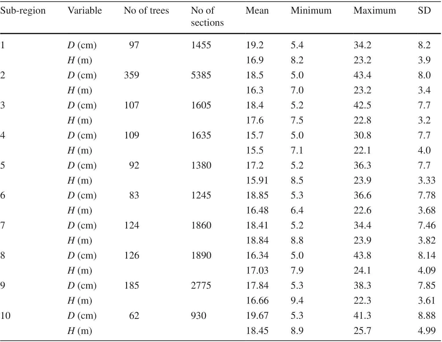
Table 1 Descriptive statistics for sample trees of 10 subregions in the Daxingan Mountains
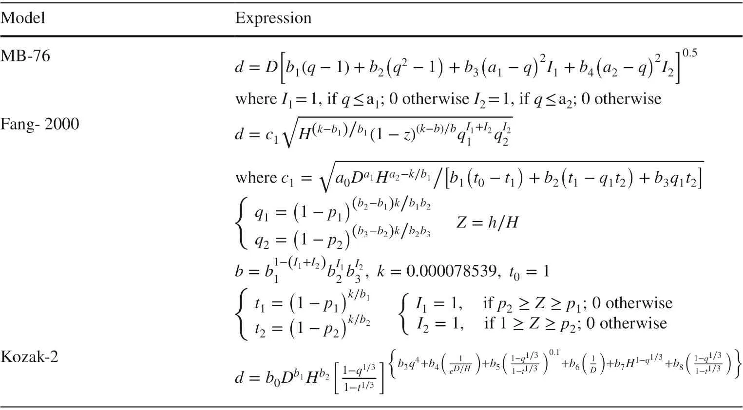
Table 2 Analyzed taper functions
Model fitting
The model parameters were estimated by the generalized non-linear least-squares methods with the MODEL procedure of SAS (SAS Institute Inc. 2008). Fitting of the stem taper equation is accompanied by various statistical problems, including lack of independence oferrors. Two additional issues of importance are multicollinearity and autocorrelation (Kozak 1997). Multicollinearity is the presence of high inter-correlations among predictor variables during the analysis of multiple regression. Dealing with excessively complicated models containing several polynomials and cross-product terms is a key reason for multicollinearity.
Autocorrelation is the occurrence of spatial correlations among the observations from the same tree that negates the assumption of independent error terms. Although leastsquares estimates of regression coeffi cients are consistent and unbiased in conjunction with multicollinearity and autocorrelation, their effi ciency is affected (Myers 1990). For this reason, suitable statistical measures need to be followed for model fitting to avoid autocorrelated errors and to reduce multicollinearity whenever possible (Kozak 1997).
The extent of multicollinearity in the models was assessed by condition number (CN), which is the square root of the quotient between maximum and minimum eigenvalues of the correlation matrix. As suggested by Myers ( 1990), a condition number greater than 1000 0.5 denotes the presence of multicollinearity- related problems. As another benchmark set by Belsley ( 1991), there should be no concern about multicollinearity, provided the CN ranges from 5–10. Multicollinearityassociated problems are formed if CN values are from 30–100 and the figure of CN from 1000–3000 signifies a high degree of multicollinearity-related problems.
During regression analysis, error terms are presumed to be independent, evenly distributed, and normal random variables (Kozak 1997). As the database for constructing taper functions consists of multiple observations pertaining to each tree, i.e., hierarchical data, it is rational to expect autocorrelation within the observations. Such correlation contravenes the assumption of independence. A continuous autoregressive error structure, CAR (1), was established to model the error terms for the adjustment of innate autocorrelation in the data. This specified error structure allows the pragmatic use of a model for unbalanced and irregularly spaced data (Gregoire et al. 1995; Dieguez-Aranda et al. 2006), both of which are attributes of many datasets in forestry (West et al. 1984).
Model comparison
The accuracy of diameter estimates for each model was judged by graphical and numerical assessment of the residuals. Two goodness-of-fit statistics, i.e., coeffi cient of determination ( R 2 ) and root mean square error ( RMSE), were tested. Some deficiencies are connected with employing R 2 in nonlinear regression, but its general expediency overrules such limitations (Thomas 1997). However, it is not advisable to use R 2 as the sole criterion while choosing the best model (Myers 1990). The use of RMSEis advantageous since its measurement units are the same as those of the dependent variable, and therefore displays the average error of a model. The notations for these statistics are as under:
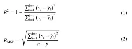

Ordinary residuals indicate the excellence of fit but these residuals will not likely measure the quality of the predictions in the future (Myers 1990). Thus, it is mandatory to validate the model and only separate data will serve the purpose to some extent. As the chances to access validation data are limited, a number of methods have been suggested, (e.g., splitting the data for fitting and validation, double cross-validation), although it is rare to obtain any additional information beyond the statistics revealed from the models fitted to the entire dataset (Kozak and Kozak 2003). Therefore, in this study, it was decided to make decisions using the available data.
The box and whisker plots of d residuals against relative heights along the stem (5%, 15%, 25% and up to 95%) were also developed to assess the suitability of taper models. These graphs illustrate the domains where the functions deliver inadequate or acceptable predictions (Kozak and Smith 1993; Kozak 2004).
Mixed-effects modeling
Since the late twentieth century, the use of mixed-effects models has become popular in forest growth and yield modeling. Compared to the regression method, these models consist of fixed and random effects parameters to account for the between-tree and within-tree variations in the data (Fang and Bailey 2001; Garber and Maguire 2003; de-Miguel et al. 2013). Additionally, this technique enables the calibration of the taper equation for a specific site or tree, provided additional measurements are available.
After selecting the best taper model, several nonlinear mixed-effects models were developed using different combinations of random parameters. The combinations of these included only those that have an effect on the parameters of the best taper model. In this study, we used the NLMIXED procedure in SAS (SAS Institute Inc. 2008) to estimate the fixed and random parameters. Mixed models were compared using Akaike’s Information Criterion (Akaike 1974), Schwarz’s Information Criterion (Schwarz 1978), and twice the negative log-likelihood, –2Ln (L). To avoid over-parameterization and convergence problems, mixed models were fitted for different sub-regions.
Comparison of taper functions among regions
The non-linear extra sum of squares method was used to find whether different taper functions would be needed for different regions (Bates and Watts 1988). In this method, fitting of full and reduced models is required. It has repeatedly been implemented to judge the necessity of separate models for specified species or distinct geographical regions, e.g., Huang et al. 2000a, b; Zhang et al. 2002; Rivas et al. 2004. The full model constitutes a separate set of parameters for each region, while the reduced model involves the same set of parameters for all regions under consideration. The full model is attained by expanding all global parameters with a dummy variable and an associated parameter to distinguish the regions. The significance of the comparison between full and reduced models is based on the F-test of the formula:

where SSER, SSEF, dfR, and dfFare the error sum of squares and degrees of freedom for reduced and full models, respectively. The non-linear extra sum of squares follows an F- distribution.
Provided the F-test reveals no differences among taper equations for different regions, a simple composite model fitted with the combined data is desired. If the F-test results indicate otherwise, i.e., taper equations are not the same across regions ( P < 0.05), more tests are needed to evaluate whether the differences are due to as few as two or as many as all of the regions. In our case, a full model for all possible sub-regions paired comparisons should be matched with the corresponding reduced model by the F-test. Taper functions for these sub-regions should be considered alike and combined in situations only when an insignificant F-value ( P > 0.005 considering the Bonferroni’s correction) is obtained.
Results
Most of the parameters were significant at P < 0.05 (Table 3, 4, 5). The exceptions were: b6for sub-regions 1 and 5; b2for sub-region 7; b4, b6for sub-regions 6 and 8; b4, b8for sub-regions 2 and 3; b2, b7, b8for sub-region 9; b6, b7, b8for sub-region 10, and b4, b6, b7, b8for sub-region 4 in the model of Kozak-2.
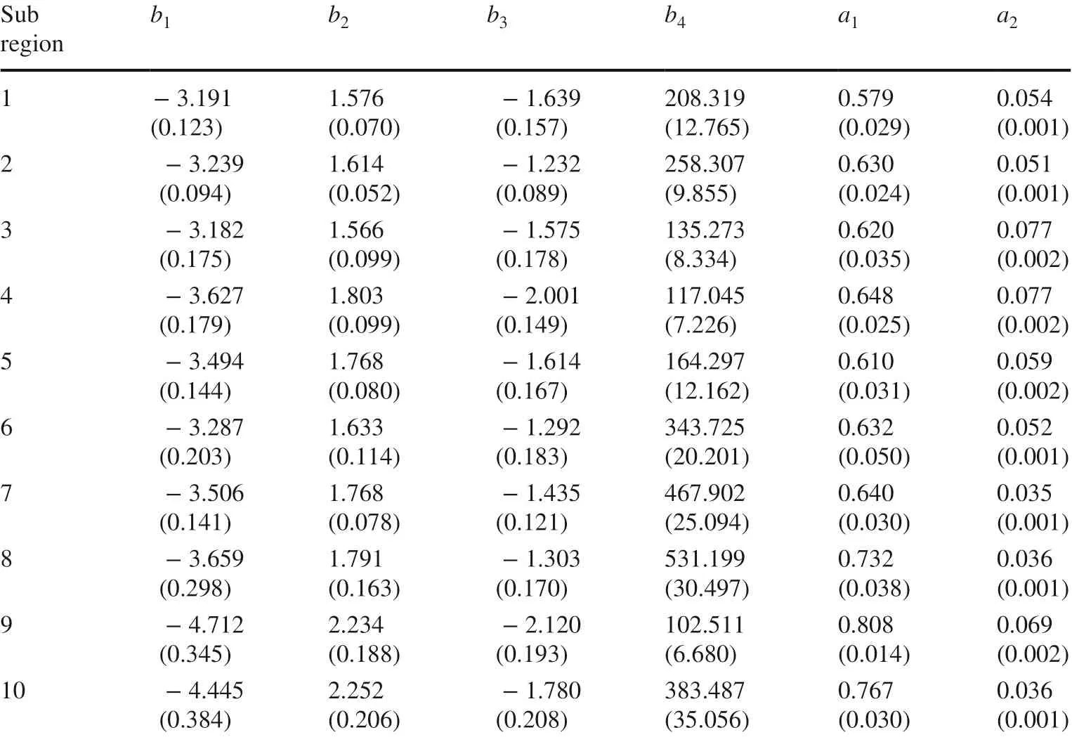
Table 3 Parameter estimates for MB-76 equation for each sub-region. Standard errors of the estimated parameters are shown in in bracket
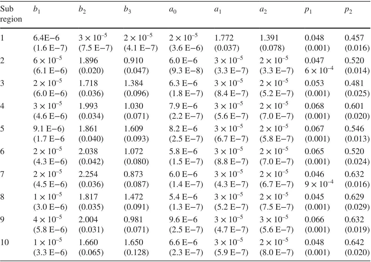
Table 4 Parameter estimates for Fang-2000 equation for each sub-region
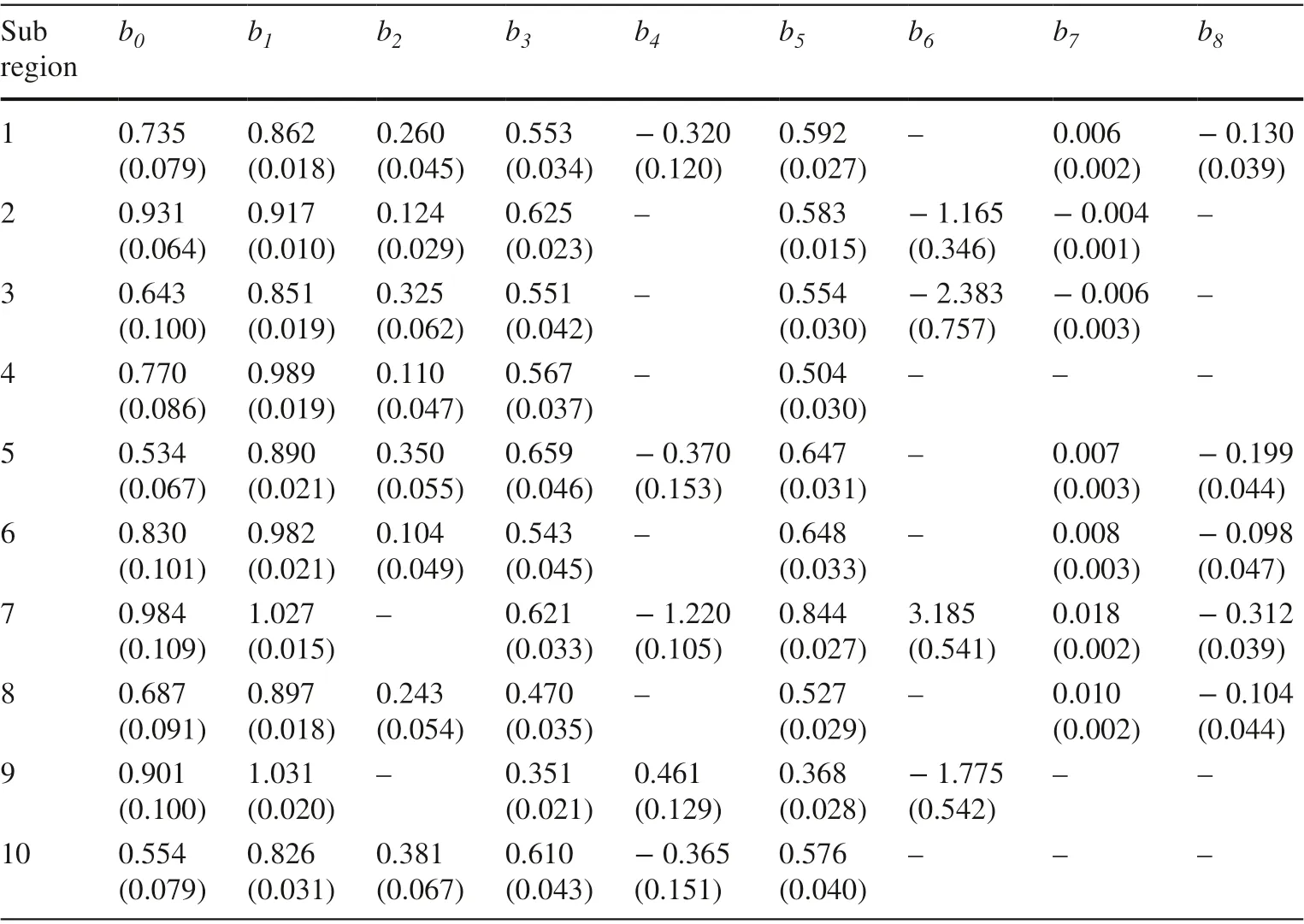
Table 5 Parameter estimates for Kozak-2 equation for each sub-region
The values of the coeffi cient of determination ( R 2 ) and root mean squared error ( RMSE) for all models are shown in Table 6. Above 98% of the total variance of d was explained by the models in seven sub-regions except subregions 3, 6, and 8, where almost 98% of the total variance was indicated. The values of RMSEvaried between 0.98 and 1.37 cm depending upon the sub-region. The model of Kozak-2 with the smallest RMSEwas the most stable taper function for all sub-regions except sub-region 4, where it was replaced by the MB-76 model. As per statistics, the leading model was Kozak-2, closely followed by MB-76. Among the three contesting models, the variability displayed by the model of Fang-2000 was relatively higher. Multicollinearity was noted in the models as implied by the condition numbers. The minimum value of CN was 38 ? 100 from the MB-76 model, followed by the values of 106 ? 152 and 70 ? 110 for the Kozak-2 and Fang-2000 models, respectively.
The box and whisker plots of d residuals versus relative height classes showed that the error was small, and its distribution along the stem was almost the same among different taper functions (Appendix Fig.S1). Plots showed overall satisfactory performance of the models and did not indicate any distinct inconsistencies among the models.
According to the fit-statistics and box plots, the models of MB-76 and Kozak-2 were more accurate than the Fang-2000 model in predicting diameters. The MB-76 equation was, however, suggested for diameter estimates due to the lowest CN and the provision of an integral solution for volume calculation. The results of the F-test of the MB-76 equation indicated consistent significant differences in different regions (not shown).
The adaptation of the MB-76 model was refitted using nonlinear mixed-effects techniques. The estimated parameters and fit statistics of the best mixed model are listed in Tables 7 and 8.
Discussion
Ample material is available on manifold functions and procedures for the precise estimation of diameter at any position along the trunk (Crecente-Campo et al. 2009; Heidarsson and Pukkala 2011; Hjelm 2013; ?zcelik and G?ceri 2015; Lumbres et al. 2016; ?zcelik and Crecente-Campo 2016; Tang et al. 2017). In this study, three stem taper functions from two groups, segmented and variable exponent, were fitted to estimate stem diameters of white birch with the best possible accuracy.
Prospective variations among the regions were examined by grouping the data into ten sub-regions for which all models were fitted independently (Table 6). As noted earlier, all models exhibited above 98% of the total variance of d accounted for in most of the sub-regions. Furtherexamination of Table 6 reveals that the models of MB-76 and Kozak-2 accounted for total variability better than the model of Fang-2000, which furnished the highest RMSEvalues. As per goodness-of-fit statistics, models of Kozak-2 and MB-76 demonstrated the lowest errors in predicting stem diameter in all regions with the model of Kozak-2 slightly ahead of MB-76. Although the prediction of merchantable or total stem volumes is beyond the scope of this study, it is important to note that variable form taper functions, to which category Kozak-2 belongs, cannot be integrated analytically. To overcome this diffi culty, integration of the taper equation is required to estimate merchantable height (Gómez-García et al. 2013). Alternatively, analytical compatibility on the part of MB-76 is a point worth noting.
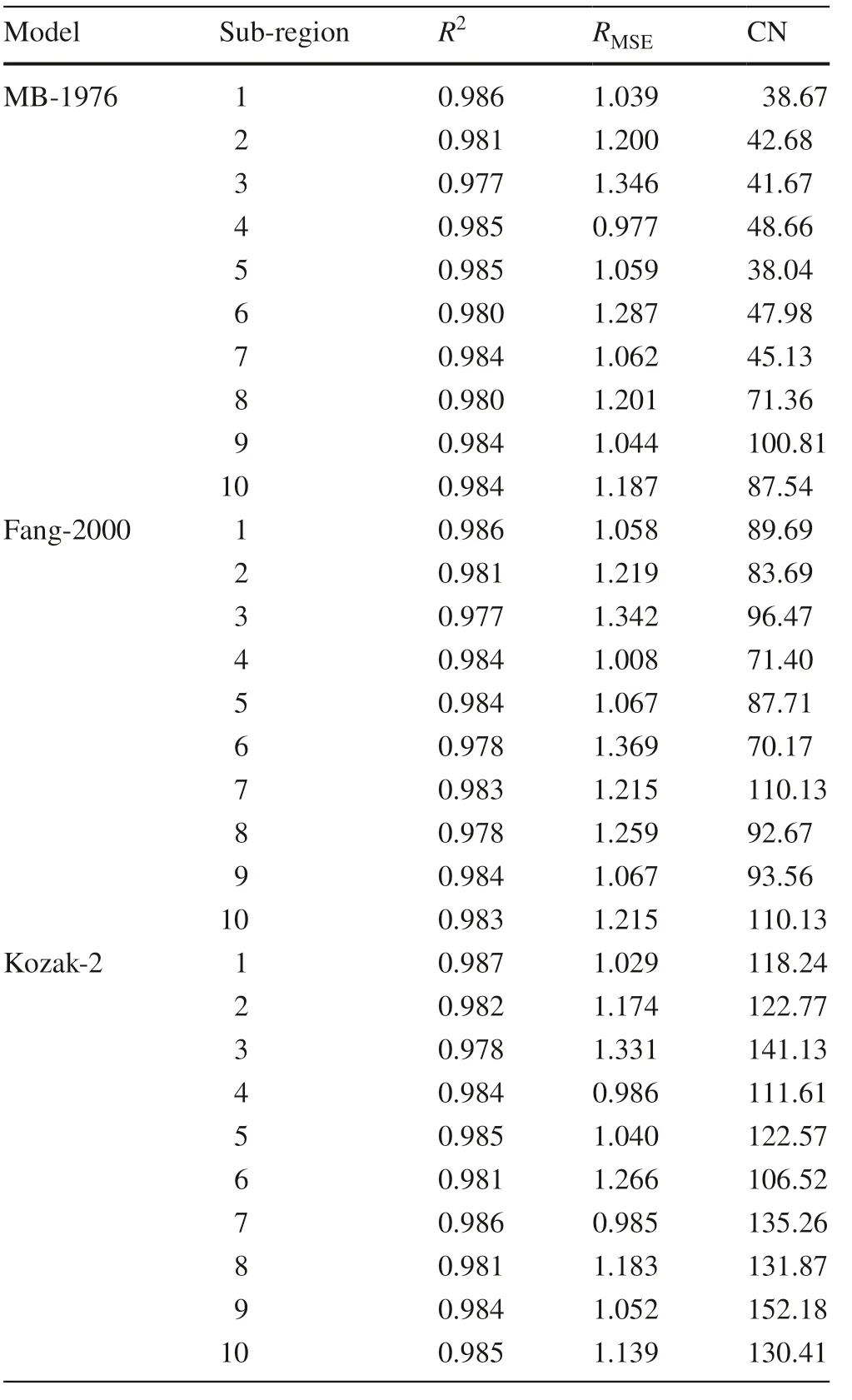
Table 6 Goodness-of-fit statistics and condition number of the taper models analyzed
The box and whisker plots provide the mean, maximum and minimum errors of prediction, median, and interquartile range (IQR) of diameter residuals by relative height classes (Appendix Fig.S1). The narrowness of IQR demonstrates that the precision of prediction is relatively high in all regions. No significant differences were displayed among the models in the plots of d residuals versus relative height classes. As a whole, all models presented higher standard errors ofestimates at 0 ? 10% and 65% ? 85% relative heights, which may be attributed to the association of these specific parts of the stem with butt swell and the point of the base of live crown (Jiang et al. 2005). The models performed well for the sections nearest the ground. Accurate diameter estimation in this section is vital considering the commercial value of the basal log.
All models portrayed similar and homogenous d residual distributions in general, as the medians are largely distributed near zero. Close observation, however, shows that the MB-76 model slightly underestimates the relative heights of 35 ? 55% of trees in sub-regions 1, 2, 3, 6, and 7 and overestimates at relative height 15 ? 25%. The middle bole sections are marginally underestimated by Kozak-2 in sub-regions 1, 2, 5, and 6, but the extent oferror is lower than the MB-76 function, as it is restricted to the 35 ? 45% relative height class. The top bole section is underestimated by Kozak-2 in all sub-regions. Being the least valued part of the stem, this error does not generally influence the performance of the models. The Fang-2000 model underestimated relative height classes 35 ? 45% in sub-regions 1, 2, 5, 6, and 7 and overestimated by 15 ? 25% in sub-regions 3 and 4. Data on all these plots were too close to decide the superiority of a model.
All models in this study are affected by multicollinearity to some extent. It is worth noting however, that the condition number (CN) of the MB-76 model is lower than for the Kozak-2 and Fang-2000 models. The minor CN value of the MB-76 model was previously noted in a stem taper study in southern China where it was as low as 7.6 (Tang et al. 2017) but still higher than the Kozak-2, Fang-2000 or other similar models (Rojo et al. 2005; Dieguez-Aranda et al. 2006; ?zcelik and Crecente-Campo 2016). The CN values are not in an acceptable range for the Kozak-2 and Fang-2000 models, as noted in earlier studies (Barrio Anta et al. 2007; Corral-Rivas et al. 2007). In terms of multicollinearity, the MB-76 model ranked best among the models in this analysis.
The fit statistics and graphic illustrations showed marginal differences between the MB-76 and Kozak-2 models. At the same time, they were more reliable than the Fang-2000 equation for the diameter estimates in all sub-regions. For the models of MB-76 and Kozak-2, the multicollinearity was significantly lower in the former. Kozak ( 1997) suggested that a model with less severe multicollinearity would be preferable. Although this analysis was limited todiameter predictions, the MB-76 equation can also provide estimates of total and merchantable volumes. Besides, this equation contains all significant parameters compared with the Kozak-2 equation. While evaluating the suitability of a model, some studies have considered the multicollinearity, compatibility, and significance of parameters, e.g., Sakici et al. 2008; Crecente-Campo et al. 2009; ?zcelik et al. 2016; Tang et al. 2017. Therefore, the MB-76 model was selected.
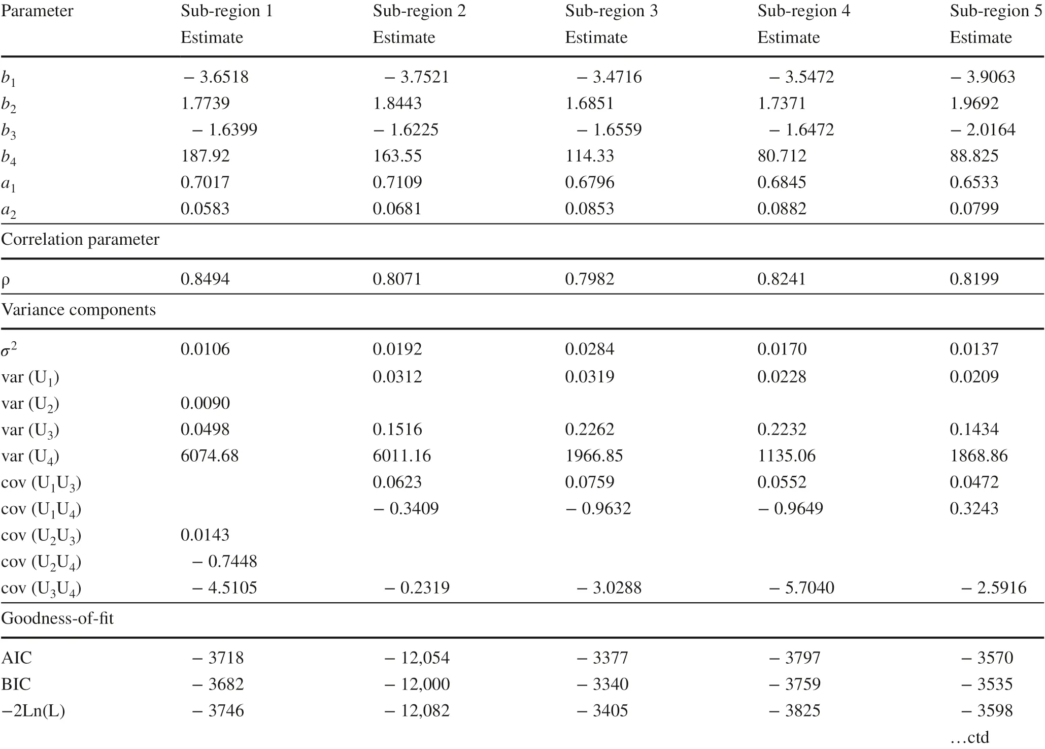
Table 7 Parameter estimates for the MB-76 model with mixed effects for sub-regions 1–5 of study area
To test the reliability ofour results, previous studies were reviewed and the MB-76 model has been popular for a variety of species (Martin 1981; Brooks et al. 2002, 2008; Jiang et al. 2005; Teshome 2005; Coble and Hilpp 2006; ?zcelik and Brooks 2012; Doyog et al. 2017). Of five equations, this model was most consistent in a study of 18 Appalachian hardwood species in predicting diameter, height, and volume (Martin 1981). As an extensively used model for the prediction of taper and volume, Coble and Hilpp ( 2006) recommended it for diameter and volume estimation of loblolly pine ( Pinus taeda L.) in East Texas, USA. In another study in northwestern Spain, it was a successful model of 14 equations analyzed for accurate diameter estimation at all positions along the stem in Scots pine plantations (Dieguez-Aranda et al. 2006). A study by Brooks et al. ( 2008), on compatible stem taper and volume equations in Turkey, found it as a reliable model for various statistical measures and sectional performance.
In some studies, the MB-76 equation was not the highest-ranking model. In appraising 33 stem taper equations, de-Miguel et al. ( 2012) found the model to be the best amongst eight equations. However, with further analysis, the MB-76 model was less accurate in volume prediction. In a comparison of several stem taper models for Lebanon cedar ( Cedrus libani A. Rich.) the model’s performance was poor in predicting diameter and other variables (?zcelik and Crecente-Campo 2016). Another comparative study of 31 taper functions for the Bornmullerian fir ( Abies nordmanniana subsp. bornmulleriana Mattf.), the MB-76 equation was third among the segmented functions(Sakici et al. 2008). These studies do not fully corroborate our findings, as taper functions are species-specific and their accuracy depends upon the particular species and its stem form (Schr?der et al. 2014).
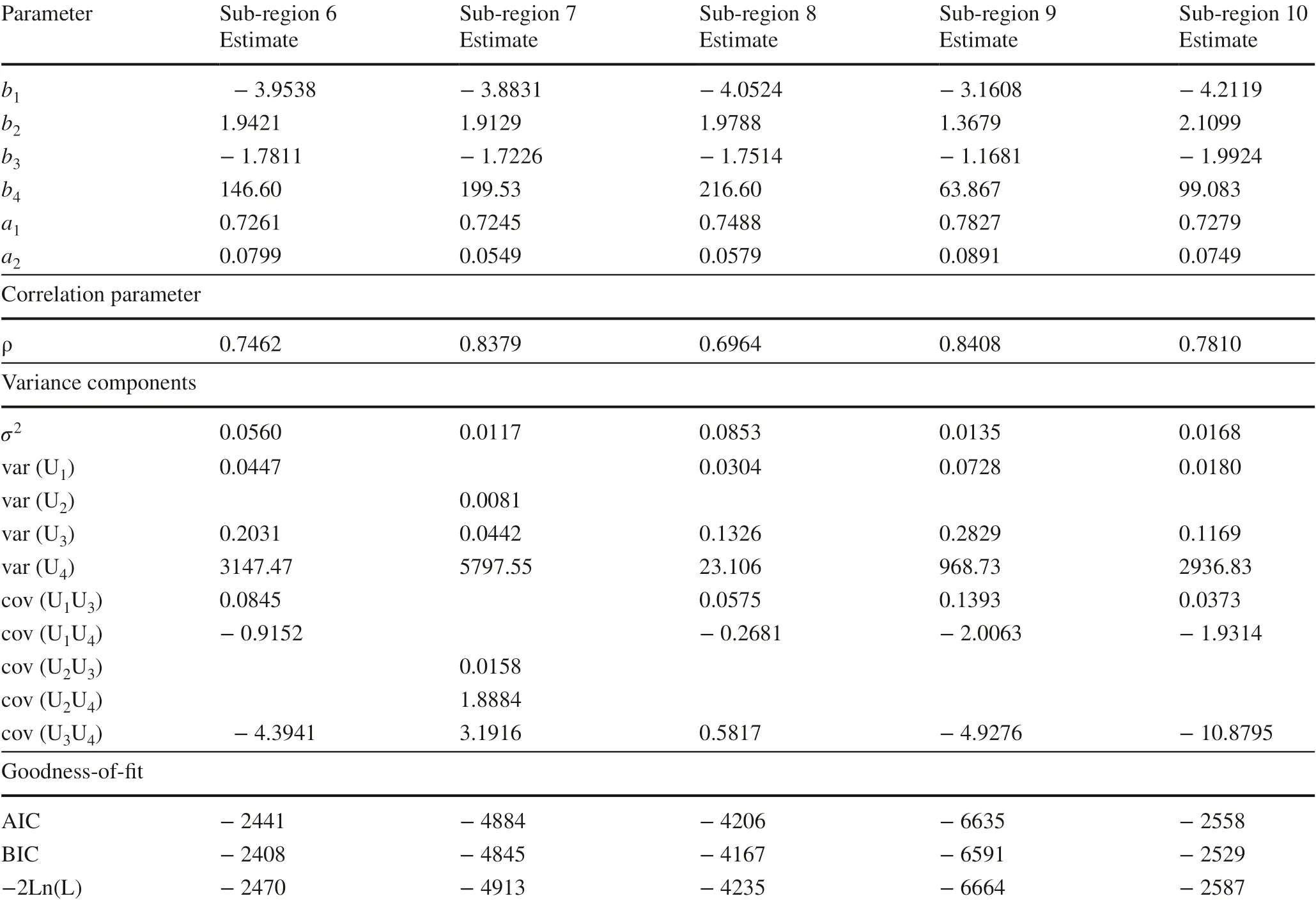
Table 8 Parameter estimates for the MB-76 model with mixed effects for sub-regions 6–10 of study area
Nonconformity ofone equation for different sub-regions was expected, due to the distinct geographical and environmental conditions in the regions.The Daxing’an Mountains extending from the northeast to southwest has different topography on eastern and western slopes; east slopes are steep and west slopes are relatively smooth (Zhang et al. 1992). There is considerable variation in temperatures and precipitation. Southern regions have higher temperatures and more precipitation, while northern areas have lower temperatures and less precipitation. Forest fires are another important ecological factor affecting natural regeneration of the birch forest. Density is increased with increasing fire intensity (Shi et al. 2010). The intensity of forest fires is also influenced by variations in topography and meteorological conditions in this region (Fan et al. 2017). Such contrasting geo-climatic factors are reflected in soil development. Lower elevations of the Daxing’an range have dark brown forest soils with high organic matter (16 ? 20%). Towards the south of the range, the brown forest soils contain less organic matter (9%). In drier and colder areas, chestnut soils are also present (Burger and Shidong 1988). Therefore, a combination of biogeoclimatic conditions determines the variations in tree taper among the sub-regions. Zhang et al. ( 2002) and ?zcelik et al. ( 2016) reported similar findings for jack pine ( Pinus banksiana Lamb.), and brutian and black pines ( Pinus brutia Ten. and Pinus nigra Arnold.) in Ontario and southern Turkey, respectively.
Similarly, some researchers have specifically investigated the effect of climate and other local factors on stem taper. Climate-induced changes in stem form were recorded for Korean red pine ( Pinus densiflora Siebold & Zucc.) in Korea (Lee et al. 2006), for lodgepole pine ( Pinus contorta Douglas) in British Columbia (Nigh and Smith 2012), and for several North American tree species (Schneider et al. 2018). Li et al. ( 2011) also found the influence ofelevation on stem taper of Schrenk’s spruce ( Picea schrenkiana Fisch. & C.A. Mey.) in northwest China. The quantification of climatic effects on stem taper was not in an objective of this study. Further research might support the decision to fit the separate models for different sub-regions.
The fixed-effects models, fitted by ordinary least squares or nonlinear least squares, minimize the sum of squared differences between the observed and predicted values of the data. The sum of squared errors is smaller than for mixedeffects models when the random parameters are not used in prediction. The fixed-effects models are more accurate when the random parameters of the mixed-effects models are supposed to be zero and additional measurements are not available to calibrate the model (Meng et al. 2009; Pukkala et al. 2009; Shater et al. 2011; Groom et al. 2012; Guzmán et al. 2012; de-Miguel et al. 2013; Arias-Rodil et al. 2015).
Consequently, for prediction purposes, many researchers suggest using the fixed-effects models in the absence of calibration data (de-Miguel et al. 2013; Arias-Rodil et al. 2015). However, de-Miguel et al. ( 2013) advised to record both fixed and mixed-effect forms of a model since calibration may be feasible in some cases. Calibration can assist in determining the best estimates with or without the prospect of model calibration. Accordingly, mixed-effects modeling of the MB-76 equation was carried out. Mixed-effects models would be used where additional upper stem diameter measurements are available for calibration.
Conclusion
Three widely used stem taper functions, Kozak-2, MB-76, and Fang-2000 were evaluated for Betula platyphylla in different sub-regions of the Daxing’an Mountains. Kozak-2 and MB-76 models provided good results and were similar to a certain extent. Without multicollinearity, Kozak-2 performed slightly better in the goodness of fit statistics and graphical representation. As recommended in the literature, models bearing less multicollinearity should be preferred. Lowest multicollinearity and all significant parameters are two substantial rationales to suggest the MB-76 model for diameter prediction of B. platyphylla in northeast China.
Open AccessThis article is licensed under a Creative Commons Attribution 4.0 International License, which permits use, sharing, adaptation, distribution and reproduction in any medium or format, as long as you give appropriate credit to the original author(s) and the source, provide a link to the Creative Commons licence, and indicate if changes were made. The images or other third party material in this article are included in the article’s Creative Commons licence, unless indicated otherwise in a credit line to the material. If material is not included in the article’s Creative Commons licence and your intended use is not permitted by statutory regulation or exceeds the permitted use, you will need to obtain permission directly from the copyright holder. To view a copy of this licence, visit http://creat iveco mmons.org/licen ses/by/4.0/.
References
Akaike H (1974) A new look at the statistical identification model. IEEE Trans Automat Control 19:716–723. https ://doi.org/10.1109/TAC.1974.11007 05
Arias-Rodil M, Diéguez-Aranda U, Rodríguez Puerta F, López-Sánchez CA, Canga Líbano E, Cámara Obregón A, Castedo-Dorado F (2015) Modelling and localizing a stem taper function for Pinus radiata in Spain. Can J For Res 45:647–658. https://doi.org/10.1139/cjfr-2014-0276
Barrio Anta M, Diéguez-Aranda U, Castedo-Dorado F, álvarez González JG, von Gadow K (2007) Merchantable volume system for pedunculate oak in northwestern Spain. Ann For Sci 64:511–520. https://doi.org/10.1051/fores t:20070 28
Bates DM, Watts DG (1988) Nonlinear regression analysis and its applications. Wiley, New York, p 365
Behre EC (1923) Preliminary notes on studies of tree form. J For 21:507–511. https://doi.org/10.1093/jof/21.5.507
Belsley DA (1991) Conditioning diagnostics: collinearity and weak data in regression. Wiley, New York, p 396
Berhe L, Arnoldsson G (2008) Tree taper models for Cupressus lusitanica plantations in Ethiopia. South For 70:193–203. https://doi.org/10.2989/Sf.2008.70.3.2.663
Brooks JR, Jiang L, Ozcelik R (2008) Compatible stem volume and taper equations for Brutian pine, Cedar of Lebanon, and Cilicica fir in Turkey. For Ecol Manage 256:147–151. https://doi.org/10.1016/j.forec o.2008.04.018
Brooks JR, Martin S, Jordan J, Sewell C (2002) Interim taper and cubic-foot volume equations for young longleaf pine plantations in southwest Georgia. In: General Technical Reports SRS–48 Asheville, NC, US Department of Agriculture, Forest Service, Southern Research Station, pp 467–470
Burger D, Shidong Z (1988) An introductory comparison of forest ecological conditions in northeast China and Ontario, Canada. For Chron 64:105–115. https://doi.org/10.5558/tfc64 105-2
Burkhart HE, Avery TE, Bullock BP (2019) Forest measurements, 6th edn. Waveland Press, Long Grove, p 434
Coble DW, Hilpp K (2006) Compatible cubic-foot stem volume and upper-stem diameter equations for semi-intensive plantation grown loblolly pine trees in East Texas. South J Appl For 30:132–141. https://doi.org/10.1093/sjaf/30.3.132
Corral-Rivas JJ, Dieguez-Aranda U, Corral Rivas S, Castedo-Dorado F (2007) A merchantable volume system for major pine species in El Salto, Durango (Mexico). For Ecol Manage 238:118–129. https://doi.org/10.1016/j.forec o.2006.09.074
Crecente-Campo F, Rojo Alboreca A, Diéguez-Aranda U (2009) A merchantable volume system for Pinus sylvestris L. in the major mountain ranges of Spain. Ann For Sci 66:808–808. https://doi.org/10.1051/fores t/20090 78
Demaerschalk JP (1972) Converting volume equations to compatible taper equations. For Sci 18:241–245. https://doi.org/10.1093/fores tscie nce/18.3.241
Demaerschalk JP, Kozak A (1977) The whole-bole system: a conditioned dual-equation system for precise prediction of tree profiles. Can J For Res 7:488–497. https ://doi.org/10.1139/x77-063
de-Miguel S, Meht?talo L, Shater Z, Kraid B, Pukkala T (2012) Evaluating marginal and conditional predictions of taper models in the absence of calibration data. Can J For Res 42:1383–1394. https://doi.org/10.1139/x2012-090
de-Miguel S, Guzmán G, Pukkala T (2013) A comparison of fixed- and mixed-effects modeling in tree growth and yield prediction of an indigenous neotropical species ( Centrolobium tomentosum) in a plantation system. For Ecol Manage 291:249–258. https://doi.org/10.1016/j.forec o.2012.11.026
Dieguez-Aranda U, Castedo-Dorado F, Alvarez-Gonzalez JG, Rojo A (2006) Compatible taper function for Scots pine plantations in northwestern Spain. Can J For Res 36:1190–1205. https://doi.org/10.1139/X06-008
Doyog ND, Lee YJ, Lee SJ, Kang JT, Kim SY (2017) Compatible taper and stem volume equations for Larix kaempferi (Japanese larch) species of South Korea. J Mt Sci 14:1341–1349. https://doi.org/10.1007/s1162 9-016-4291-x
Fan Q, Wang C, Zhang D, Zang S (2017) Environmental influences on forest fire regime in the Greater Hinggan mountains, northeast China. Forests 8:1–16. https://doi.org/10.3390/f8100 372
Fang Z, Bailey RL (2001) Nonlinear mixed effects modeling for slash pine dominant height growth following intensive silvicultural treatments. For Sci 47:287–300. https://doi.org/10.1093/fores tscie nce/47.3.287
Fang Z, Borders BE, Bailey RL (2000) Compatible volume-taper models for loblolly and slash pine based on a system with segmented-stem form factors. For Sci 46:1–12. https ://doi.org/10.1093/fores tscie nce/46.1.1
Far-East-American (2012) White birch plywood. https ://www.feaco .com/produ cts/impor ted-hardw ood-plywo od/white -birch /. Accessed 25 Oct 2017
Fonweban J, Gardiner B, Macdonald E, Auty D (2011) Taper functions for Scots pine ( Pinus sylvestris L.) and sitka spruce ( Picea sitchensis (Bong.) Carr.) in Northern Britain. Forestry 84:49–60. https://doi.org/10.1093/fores try/cpq04 3
Garber SM, Maguire DA (2003) Modeling stem taper of three central Oregon species using nonlinear mixed effects models and autoregressive error structures. For Ecol Manage 179:507–522
Gregoire TG, Schabenberger O, Barrett JP (1995) Linear modelling of irregularly spaced, unbalanced, longitudinal data from permanent-plot measurements. Can J For Res 25:137–156. https://doi.org/10.1139/x95-017
Groom JD, Hann DW, Temesgen H (2012) Evaluation of mixed-effects models for predicting Douglas-fir mortality. For Ecol Manage 276:139–145. https://doi.org/10.1016/j.forec o.2012.03.029
Guzmán G, Pukkala T, Palahí M, de-Miguel S, (2012) Predicting the growth and yield of Pinus radiata in Bolivia. Ann For Sci 69:335–343. https://doi.org/10.1007/s1359 5-011-0162-3
Gál J, Bella IE (1994) New stem taper functions for 12 Saskatchewan timber species, Information Report (NoFC-Edmonton). Canadian Forest Service, Northern Forestry Centre, Alberta, pp 1–25
Gómez-García E, Crecente-Campo F, Diéguez-Aranda U (2013) Selection of mixed-effects parameters in a variable–exponent taper equation for birch trees in northwestern Spain. Ann For Sci 70:707–715. https://doi.org/10.1007/s1359 5-013-0313-9
Heidarsson L, Pukkala T (2011) Taper functions for lodgepole pine ( Pinus contorta) and Siberian larch ( Larix sibirica) in Iceland. Icelandic Agr Sci 24:3–11
Hjelm B (2013) Stem taper equations for poplars growing on farmland in Sweden. J For Res 24:15–22. https://doi.org/10.1007/s1167 6-012-0270-4
Huang S, Price D, Titus S (2000a) Development ofecoregion-based height–diameter models for white spruce in boreal forests. For Ecol Manage 129:125–141. https ://doi.org/10.1016/S0378 -1127(99)00151-6
Huang S, Price D, Morgan D, Peck K (2000b) Kozak’s variable-exponent taper equation regionalized for white spruce in Alberta. West J App For 15:75–85. https://doi.org/10.1093/wjaf/15.2.75
Jiang L, Brooks JR, Wang J (2005) Compatible taper and volume equations for yellow-poplar in West Virginia. For Ecol Manage 213:399–409. https://doi.org/10.1016/j.forec o.2005.04.006
Jiang L, Liu R (2011) Segmented taper equations with crown ratio and stand density for Dahurian Larch ( Larix gmelinii) in Northeastern China. J For Res 22:347. https://doi.org/10.1007/s1167 6-011-0178-4
Kozak A (1988) A variable-exponent taper equation. Can J For Res 18:1363–1368. https://doi.org/10.1139/x88-213
Kozak A (1997) Effects of multicollinearity and autocorrelation on the variable-exponent taper functions. Can J For Res 27:619–629. https://doi.org/10.1139/x97-011
Kozak A (2004) My last words on taper equations. For Chron 80:507–515. https://doi.org/10.5558/tfc80 507-4
Kozak A, Kozak R (2003) Does cross validation provide additional information in the evaluation of regression models? Can J For Res 33:976–987. https://doi.org/10.1139/x03-022
Kozak A, Munro DD, Smith JHG (1969) Taper functions and their application in forest inventory. For Chron 45:278–283. https://doi.org/10.5558/tfc45 278-4
Kozak A, Smith JHG (1993) Standards for evaluating taper estimating systems. For Chron 69:438–444. https://doi.org/10.5558/tfc69 438-4
Lee WK, Biging GS, Son Y, Byun WH, Lee KH, Son YM, Seo JH (2006) Geostatistical analysis of regional differences in stem taper form of Pinus densiflora in central Korea. Ecol Res 21:513–525. https://doi.org/10.1007/s1128 4-006-0152-3
Lee WK, Seo JH, Son YM, Lee KH, von Gadow K (2003) Modeling stem profiles for Pinus densiflora in Korea. For Ecol Manage 172:69–77. https://doi.org/10.1016/S0378-1127(02)00139-1
Li LP, Wang XP, Stefan Z, Zhang LY, Fang JY (2011) Altitudinal patterns of stand structure and herb layer diversity of Picea schrenkiana forests in the central Tianshan Mountains, Northwest China. J Arid Land 3:254–260. https ://doi.org/10.3724/sp.j.1227.2011.00254
Li R, Weiskittel AR (2010) Comparison of model forms for estimating stem taper and volume in the primary conifer species of the North American Acadian Region. Ann For Sci 67:302–302. https://doi.org/10.1051/fores t/20091 09
Li R, Weiskittel A, Dick AR, Kershaw JA Jr, Seymour RS (2012) Regional stem taper equations for eleven conifer species in the Acadian Region of North America: development and assessment. North J Appl For 29:5–14
Lumbres RIC, Abino AC, Pampolina NM, Calora FG, Lee YJ (2016) Comparison of stem taper models for the four tropical tree species in Mount Makiling, Philippines. J Mt Sci 13:536–545. https://doi.org/10.1007/s1162 9-015-3546-2
Martin AJ (1981) Taper and volume equations for selected Appalachian hardwood species. USDA Forest Service, Res Pap NE-490
Matte L (1949) The taper of coniferous species with special reference to loblolly pine. For Chron 25:21–31. https ://doi.org/10.5558/tfc25 021-1
Max TA, Burkhart HE (1976) Segmented polynomial regression applied to taper equations. For Sci 22:283–289. https ://doi.org/10.1093/fores tscie nce/22.3.283
Meng SX, Huang S, Yang Y, Trincado G, VanderSchaaf CL (2009) Evaluation of population-averaged and subject-specific approaches for modeling the dominant or codominant height of lodgepole pine trees. Can J For Res 39:1148–1158. https://doi.org/10.1139/X09-039
Myers RH (1990) Classical and modern regression with applications, 2nd edn. Duxbury Press, Belmont
Nigh G, Smith W (2012) Effect of climate on lodgepole pine stem taper in British Columbia, Canada. Forestry 85:579–587. https://doi.org/10.1093/fores try/cps06 3
Osumi S (1959) Studies on the stem form of the forest trees (1) on the relative stem form. J Jpn For Soc 41:471–479. https://doi.org/10.11519/jjfs1 953.41.12_471
?zcelik R, Brooks JR (2012) Compatible volume and taper models for economically important tree species of Turkey. Ann For Sci 69:105–118. https://doi.org/10.1007/s1359 5-011-0137-4
?zcelik R, Crecente-Campo F (2016) Stem taper equations for estimating merchantable volume of Lebanon cedar trees in the Taurus Mountains, Southern Turkey. For Sci 62:78–91. https://doi.org/10.5849/forsc i.14-212
?zcelik R, G?ceri MF (2015) Compatible merchantable stem volume and taper equations for eucalyptus plantations in the Eastern Mediterranean Region of Turkey. Turk J Agri For 39:851–863. https://doi.org/10.3906/tar-1501-27
?zcelik R, Brooks JR, Jiang L (2011) Modeling stem profile of Lebanon cedar, Brutian pine, and Cilicica fir in Southern Turkey using nonlinear mixed-effects models. Eur J For Res 130:613–621. https ://doi.org/10.1007/s1034 2-010-0453-5
?zcelik R, Karatepe Y, Gürlevik N, Ca?ellas I, Crecente-Campo F (2016) Development ofecoregion-based merchantable volume systems for Pinus brutia Ten. and Pinus nigra Arnold. in southern Turkey. J For Res 27:101–117. https://doi.org/10.1007/s1167 6-015-0147-4
Pang L, Ma Y, Sharma PR, Rice S, Song X, Fu L (2016) Developing an improved parameter estimation method for the segmented taper equation through combination of constrained two-dimensional optimum seeking and least square regression. Forests 7:1–20. https://doi.org/10.3390/f7090 194
Pompa-García M, Corral-Rivas JJ, Hernández-Díaz JC, Alvarez-González JG (2009) A system for calculating the merchantable volume ofoak trees in the northwest of the state of Chihuahua. Mexico J For Res 20(4):293–300. https://doi.org/10.1007/s1167 6-009-0051-x
Pukkala T, L?hde E, Laiho O (2009) Growth and yield models for uneven-sized forest stands in Finland. For Ecol Manage 258:207–216. https://doi.org/10.1016/j.forec o.2009.03.052
Rivas JJC, Gonzalez JGL, Gonzalez ADR, von Gadow K (2004) Compatible height and site index models for five pine species in El Salto, Durango (Mexico). For Ecol Manage 201:145–160. https ://doi.org/10.1016/j.forec o.2004.05.060
Rojo A, Perales X, Sanchez-Rodriguez F, Alvarez-Gonzalez JG, von Gadow K (2005) Stem taper functions for maritime pine ( Pinus pinaster Ait.) in Galicia (Northwestern Spain). Eur J For Res 124:177–186. https://doi.org/10.1007/s1034 2-005-0066-6
SAS Institute Inc (2008) SAS/STAT? 9.2 User’s Guide. SAS Institute Inc., Cary, p 2876
Sakici OE, Misir N, Yavuz H, Misir M (2008) Stem taper functions for Abies nordmanniana subsp. bornmulleriana in Turkey. Scand J For Res 23:522–533. https://doi.org/10.1080/02827 58080 25524 53
Samuelsson F (2006) The potential for quality production in birch stands in north-eastern China using different precommercial thinning strategies (M.Sc thesis). Alnarp: SLU, Southern Swedish Forest Research Centre, p 29
Schneider R, Franceschini T, Fortin M, Saucier JP (2018) Climateinduced changes in the stem form of 5 North American tree species. For Ecol Manage 427:446–455. https://doi.org/10.1016/j.forec o.2017.12.026
Schr?der T, Costa EA, Valério AF, dos Santos LG (2014) Taper equations for Pinus elliottii Engelm. in southern Paraná. Brazil For Sci 61:311–319. https://doi.org/10.5849/forsc i.14-054
Schwarz G (1978) Estimating the dimension of a model. Ann Stat 6:461–464. https://doi.org/10.1214/aos/11763 44136
Sevillano-Marco E, Fernandez-Manso A, Castedo-Dorado F (2009) Development and applications of a growth model for Pinus radiata D. Don plantations in El Bierzo (Spain). For Syst 18:64–80. https://doi.org/10.5424/fs/20091 81-01051
Sharma M, Zhang SY (2004) Variable-exponent taper equations for jack pine, black spruce, and balsam fir in eastern Canada. For Ecol Manage 198:39–53. https://doi.org/10.1016/j.forec o.2004.03.035
Shater Z, de-Miguel S, Kraid B, Pukkala T, Palahí M (2011) A growth and yield model for even-aged Pinus brutia Ten. stands in Syria. Ann For Sci 68:149–157. https://doi.org/10.1007/s1359 5-011-0016-z
Shi F, Sasa K, Koike T (2010) Characteristics of larch forests in Daxingan Mountains, northeast China. In: Osawa A, Zyryanova O, Matsuura Y, Kajimoto T, Wein R (eds) Permafrost ecosystems. Ecological studies (analysis and synthesis), vol 209. Springer, Dordrecht, pp 367–383209
Subedi N, Sharma M, Parton J (2011) Effects of sample size and tree selection criteria on the performance of taper equations. Scand J For Res 26:555–567. https ://doi.org/10.1080/02827 581.2011.58367 7
Tang X, Pérez-Cruzado C, Fehrmann L, álvarez-González JG, Lu Y, Kleinn C (2016) Development of a compatible taper function and stand-level merchantable volume model for Chinese Fir plantations. PLoS ONE 11:e0147610. https://doi.org/10.1371/journ al.pone.01476 10
Tang C, Wang CS, Pang SJ, Zhao ZG, Guo JJ, Lei YC, Zeng J (2017) Stem taper equations for Betula alnoides in South China. J Trop For Sci 29:80–92
Teshome T (2005) Compatible volume-taper equations for predicting merchantable volume to variable merchantable limits for Cupressus lusitanica, Ethiopia. Ethiop J Sci 28:15–22. https ://doi.org/10.4314/sinet.v28i1.18227
Thomas PR (1997) Modern regression methods. Wiley, New York, p 515
Trincado G, Burkhart HE (2006) A generalized approach for modeling and localizing stem profile curves. For Sci 52:670–682. https://doi.org/10.1093/fores tscie nce/52.6.670
West PW, Ratkowsky DA, Davis AW (1984) Problems of hypothesis testing of regressions with multiple measurements from individual sampling units. For Ecol Manage 7:207–224. https://doi.org/10.1016/0378-1127(84)90068-9
Xu H, Liu Y, Jiang J, Liu G, Zhao X (2016) Progeny test of tetraploid Betula platyphylla and preliminary selection of hybrid parents. J For Res 27:665–674. https://doi.org/10.1007/s1167 6-015-0202-1
Xu J, Xie S, Han A, Rao R, Huang G, Chen X, Hu J, Liu Q, Yang X, Zhang L (2019) Forest resources in China—The 9th National Forest Inventory. National Forestry and Grassland Administration, Beijing, p 29
Zeng W, Tomppo E, Healey SP, Gadow KV (2015) The national forest inventory in China: history-results-international context. For ecosyst 2:23. https://doi.org/10.1186/s4066 3-015-0047-2
Zhang L, Peng C, Huang S, Zhou X (2002) Development and evaluation ofecoregion-based jack pine height-diameter models for Ontario. For Chron 78:530–538. https ://doi.org/10.5558/tfc78 530-4
Zhang WR, Sheng WT, Jiang YX, Zhou ZX, Wang XS (1992) Classification of forest site system in China. For Res 5:251–262 (in Chinese)
Zheng C, Wang Y, Jia L, Mason EG, We S, Sun C, Duan J (2017) Compatible taper-volume models of Quercus variabilis Blume forests in north China. iForest Biogeosci For 10:567
Zianis D, Muukkonen P, Makipaa R, Mencuccini M (2005) Biomass and stem volume equations for tree species in Europe. Silva Fenn Monogr 4:63
 Journal of Forestry Research2021年2期
- Journal of Forestry Research的其它文章
- Leaf phenotypic variation of endangered plant Tetracentron sinense Oliv. and influence of geographical and climatic factors
- Ecological variations of woody species along an altitudinal gradient in the Qinling Mountains of Central China: area-based versus mass-based expression of leaf traits
- Variations in stem radii of Larix principis-rupprechtii to environmental factors at two slope locations in the Liupan Mountains, northwest China
- A review of ecological mechanisms for management practices of protective forests
- Variation of basic density, calorific value and volumetric shrinkage within tree height and tree age of Ugandan grown Eucalyptus grandis wood
- Natural variations in flavonoids and triterpenoids of Cyclocarya paliurus leaves
