Thermodynamics of warm axionic Abelian gauge inflation
Xi-Bin Li(李喜彬) and Yan-Ling Wu(武燕玲)
1College of Physics and Electronic Information,Inner Mongolia Normal University,Hohhot 010022,China
2Inner Mongolia Key Laboratory for Physics and Chemistry of Functional Materials,Inner Mongolia Normal University,Hohhot 010022,China
Keywords: axion inflation,thermodynamics
1.Introduction
The inflation model is established to overcome some defects of the standard big bang theory.[1–4]This model has successfully answered the problems like the formation of cosmic large-scale structure[5–7]and the anisotropy of microwave background,[8–10]but come problems that, in cold inflation,the inflaton does not interact with other fields and the Universe is required a reheating process after inflation when the scalar field reaches the bottom of the potential and starts oscillating.However, this puts forward higher requirements for the potential and the reheating itself may also face some problems.Furthermore, the latest Planck data ruled out many forms of inflation potentials, including the quadratic and quartic potentials,both widely accepted from the perspective of particle physics.[11]
On the other hand, the warm inflation model was proposed as a candidate scenario to solve the problems in cold inflation.[12,13]Warm inflation has been studied for a long time as a possible and realizing model.[14–16]In warm inflationary scenario, the evolution of the inflaton field can be properly determined in the context of the in-in formalism,or Schwinger closed-time path functional formalism.[17]This formalism leads an stochastic differential equation which contains a dissipative term and a Gaussian stochastic noise term as a type of generalized Langevin-like equation of motion.[18,19]
Inflation driven by an axion-like particle,often dubbed as natural inflation,[20,21]is one of the most well-motivated models of inflation to reheat the Universe.[22]In axion inflation the flatness of the potential is guaranteed by the shift symmetry and ensures a potential periodic.However, this model in cold inflation is strongly disfavored by Planck 2018 data.[23]Another objective in cold inflation is the realization of an exponential production of radiation in order to overcome the exponential dilution without spoiling the slow-roll stage.For this purpose, the thermalized axion inflation model is introduced,in which the gauge fieldsAμsimply couple to an axionlike fieldφand the gauge fields are considered as the thermal bath.[24]In this model, inflation often follows a kination era
where the Universe is then dominated by the kinetic energy of inflaton,which suppresses the generation of radiation field and may need a long time to transit from inflation to radiation domination.On the contrary,warm inflation allows a dissipative term?˙φin the equation of motion of inflaton,which represents the decay from inflaton to thermal bath.Thus the combination of axion inflation and warm inflation is a reasonable arrangement, and this model is also called the minimal warm inflation.[25–28]Warm axion inflation allows inflaton to decay into gauge field at any time and make it possible to analyze the thermodynamics of the early Universe.The strong coupling(or strong dissipative effect)can effectively restrain the conversion to kinetic energy,thus avoiding the kination era and realizing the exponential production of thermal bath.Most importantly, warm inflationary scenario makes the pseudoscalar inflation model compatible with the Planck 2018 results.[29]
So far, there have been enough discussions on the self consistency and rationality of the warm inflation theory, but further research on thermal effect,directly related to the thermal effect, still needs to be conducted in depth.The thermal quantityTmake it possible to provide a detailed analysis on the thermal properties during and after inflation.In this paper,by starting from the Langevin equation, inflationary spectral index is analytically calculated in the model of warm axionic Abelian gauge inflation.The equation about the ratio of Hubble parameter to cosmic temperatureH/Tis obtained, thenH/TandTare numerical solved.This work provides a new scheme for the study of the thermodynamics in the early Universe, especially the evolution of temperature, and also provides a new idea for the discussion of the reheating process.
The organization of this paper is as follows: In Section 2,the spectral index is calculated from the Langevin equation in the framework of warm axion inflation.In Section 3, equations related to thermal effect,especially the cosmic temperatureT,are calculated theoretically.Then,numerical results are obtained in Section 3 and discussed in detail.Finally,in Section 4, we conclude our work and give some outlooks about our further research.
2.Spectral index of minimal warm inflation
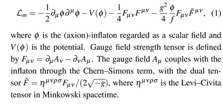
We consider the model described by the following matter Lagrangian:[30]
2.1.Perturbed dynamics
In the warm inflation model, the dynamical equation of inflaton is described by an additional dissipative term?.We define a new variable as the ratio of dissipative coefficient to the Hubble parameterQ=?/3H,such that
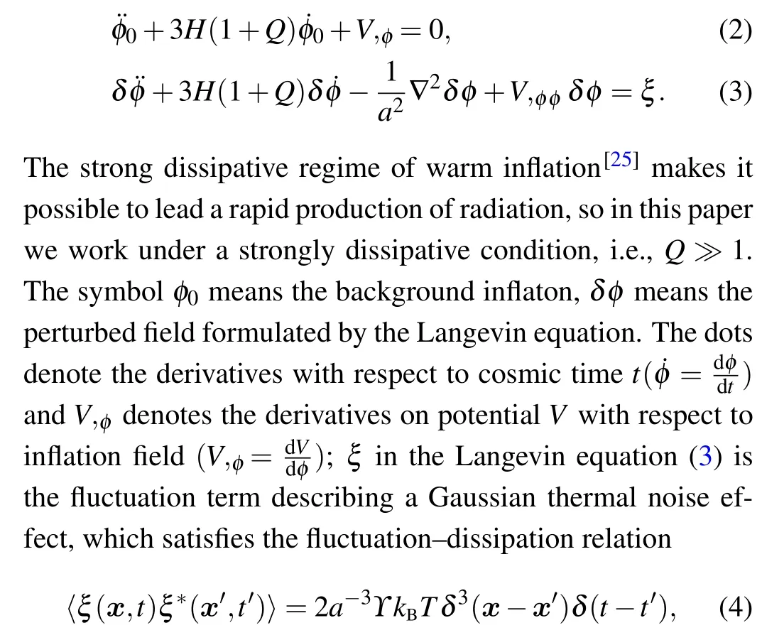
whose Fourier transformation reads

where the Planck mass is defined asM2p=1/(8πG).
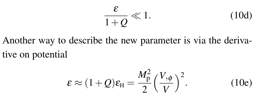
To characterize the dynamical and thermal properties of inflation,it is necessary to define three slow-roll parameters
The first slow-roll parameter in Eq.(10)means a nearly exponential expansion of the early Universe,the second one means the requirement on the flatness of potential in terms of inflaton,and the third one is required from the restriction of dissipative coefficient and potential on the inflaton derivative,namely the adiabatic approximation.Here, independent dissipative coefficientφmeansβ=0.In the following calculations,another more important slow-roll parameterε ≡QεHwill be used by satisfying the approximation
The fact that potential contributes the most of the total energy density during inflation helps us to simplify the above dynamical equations to
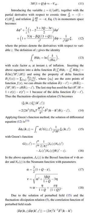
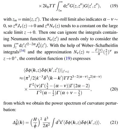
2.2.Spectral index
The spectral index of curvature perturbation is defined as
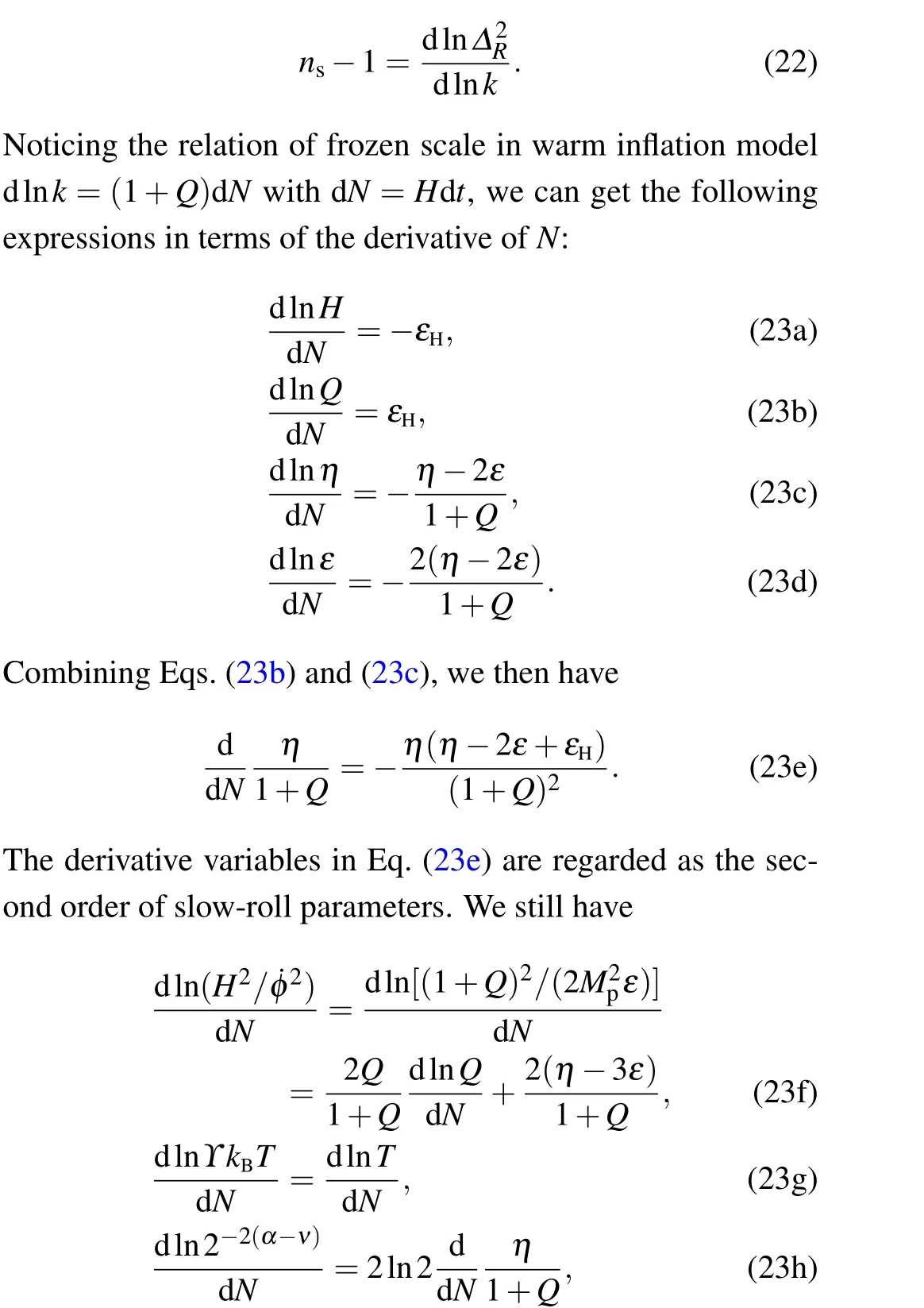
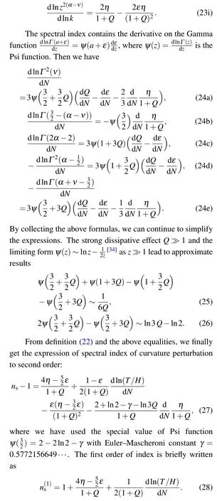
It is thus clear that if we get the expression ofH/T,the spectral index will be determined.Next,this problem will be discussed in detail.
3.Thermodynamics of radiation field
A safe way to reheat the Universe is through the couplings of inflatonφand gauge fields.Generally, the gauge boson field is regarded as the thermal bath.This model is used to explain the reheating problem in cold inflation scenario with natural and quadratic potential[22,24]and to analysis the thermal effects in warm inflation scenario,[28]then we continue the studies about inflationary thermodynamic problems in such a model.The model described by Eq.(1) shows a decay process from inflatonφto thermalizedU(1) gauge fieldAμ, in which we can calculate the energy density of radiation during inflation.
In this section, the metric is set d2s=a2(-d2τ+d2x+d2y+d2z)with conformal time dτ=dt/a.
3.1.Dynamical solution of gauge field
The equation of motion of 4-potentialAμare obtained by varying the action(1)with respect toAμ,

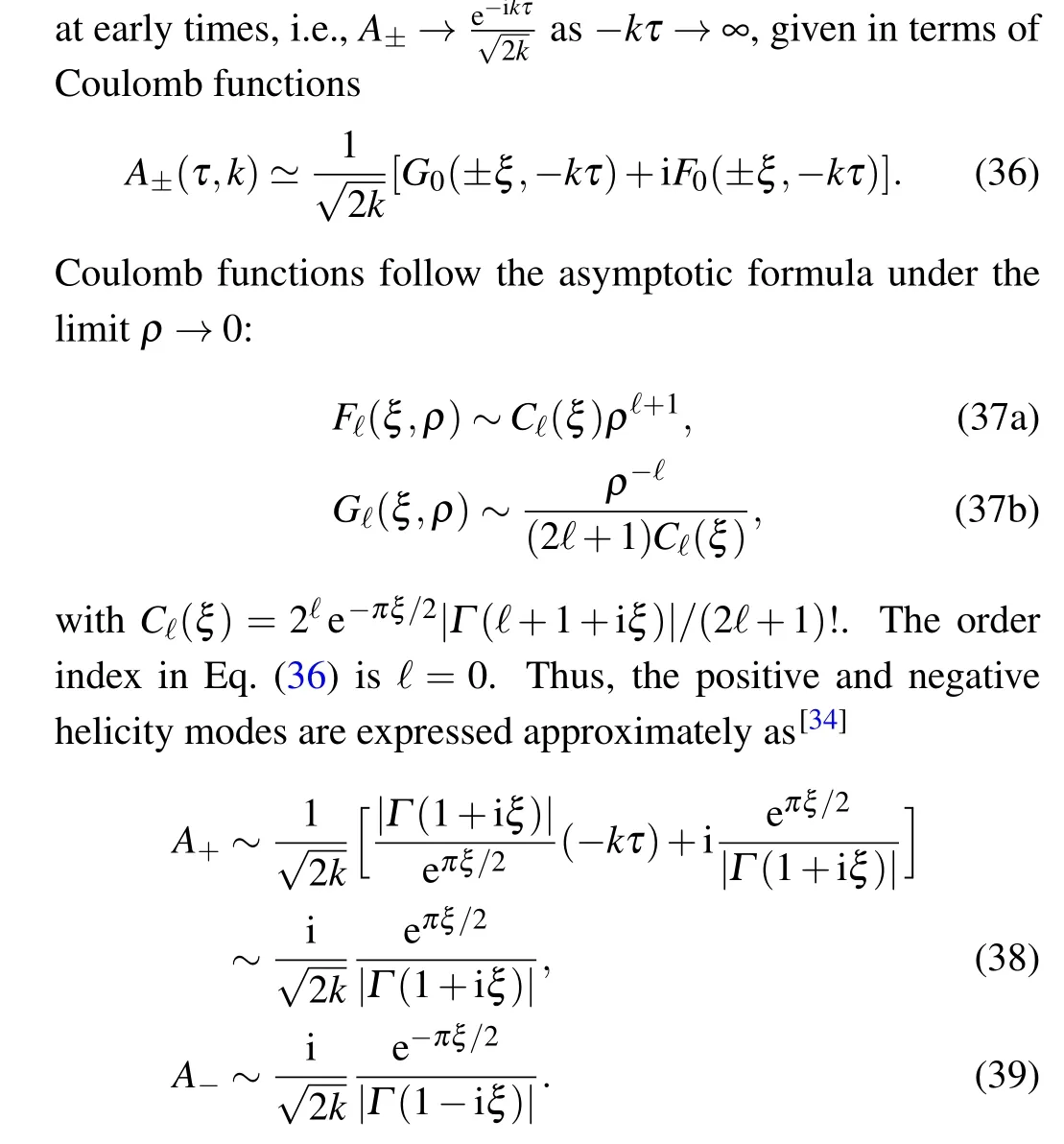
3.2.Energy density of radiation field
Spatial components of electric and magnetic fields are given by
In the above equations, dρB(k,τ)/dlnkdenotes the spectral energy density of magnetic field andPB,i jis the two-point correlation function in momentum space,with
The hyperbolic cotangent comes from the ensemble average of creation and annihilation operators.[35]In the same way the correlation function of electric field is defined.The following equalities may be helpful to calculate the correlation functions:The numerical result shows that the magnetic spectral density is at least 103times the value of electric spectral density for any value ofξ, so we can ignore the latter directly.Then the spectral density of radiation field finally arrives at
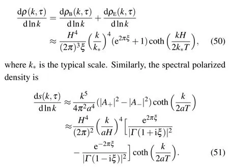
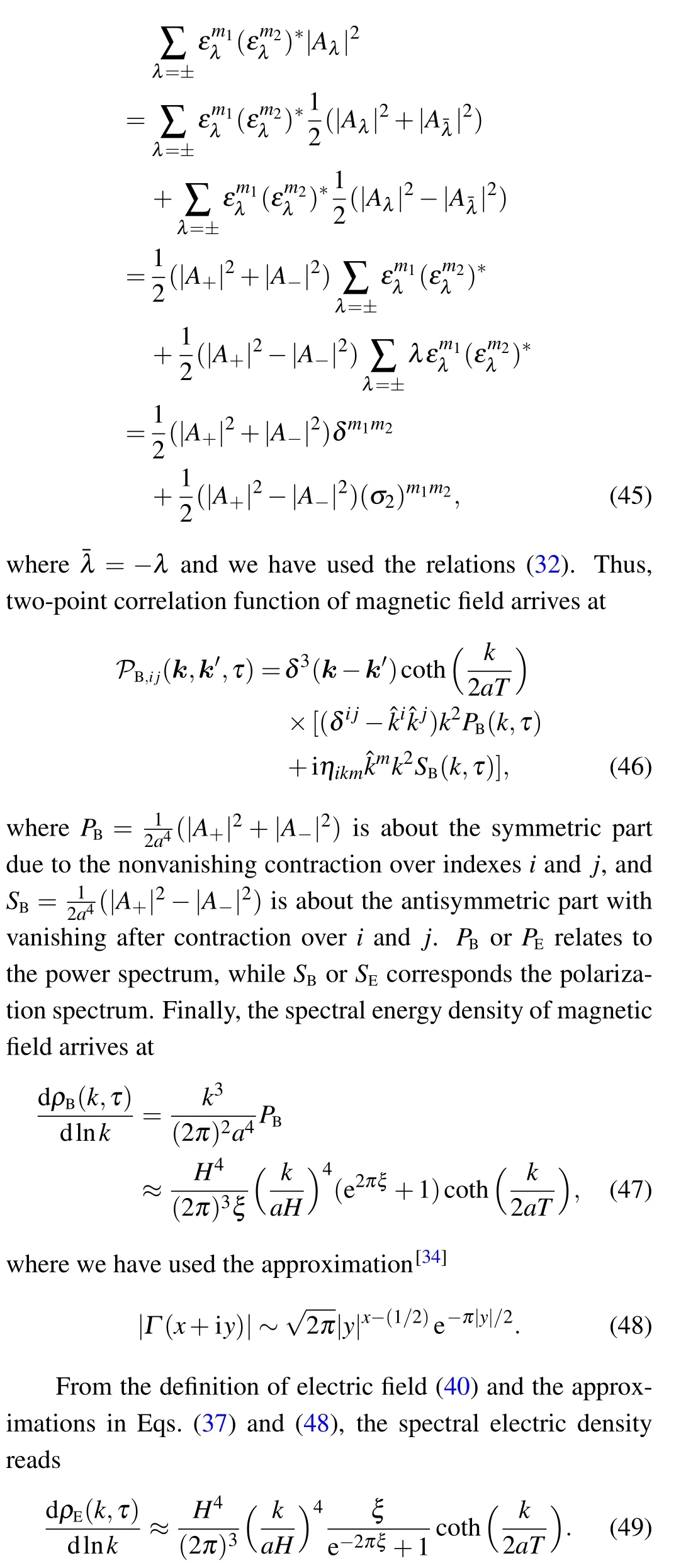
Figure 1 plots the spectral energy density in Eq.(50)and polarized density in Eq.(51)of primordial radiation field,where the wave numberkworks at the typical scalek=k*and the number related to the slow-roll parameter assignsε1/2/(1+Q)=10-3.It is found that the spectral energy density is almost independent ofξ0whenξ0<104,which means that we cannot restrict the parameters of the Chern–Simons model in Eq.(1)only by the amplitude of primordial electromagnetic field.From the perspective of observational cosmology, only the observation on energy density spectrum is not enough, but also the observation on polarized density spectrum.
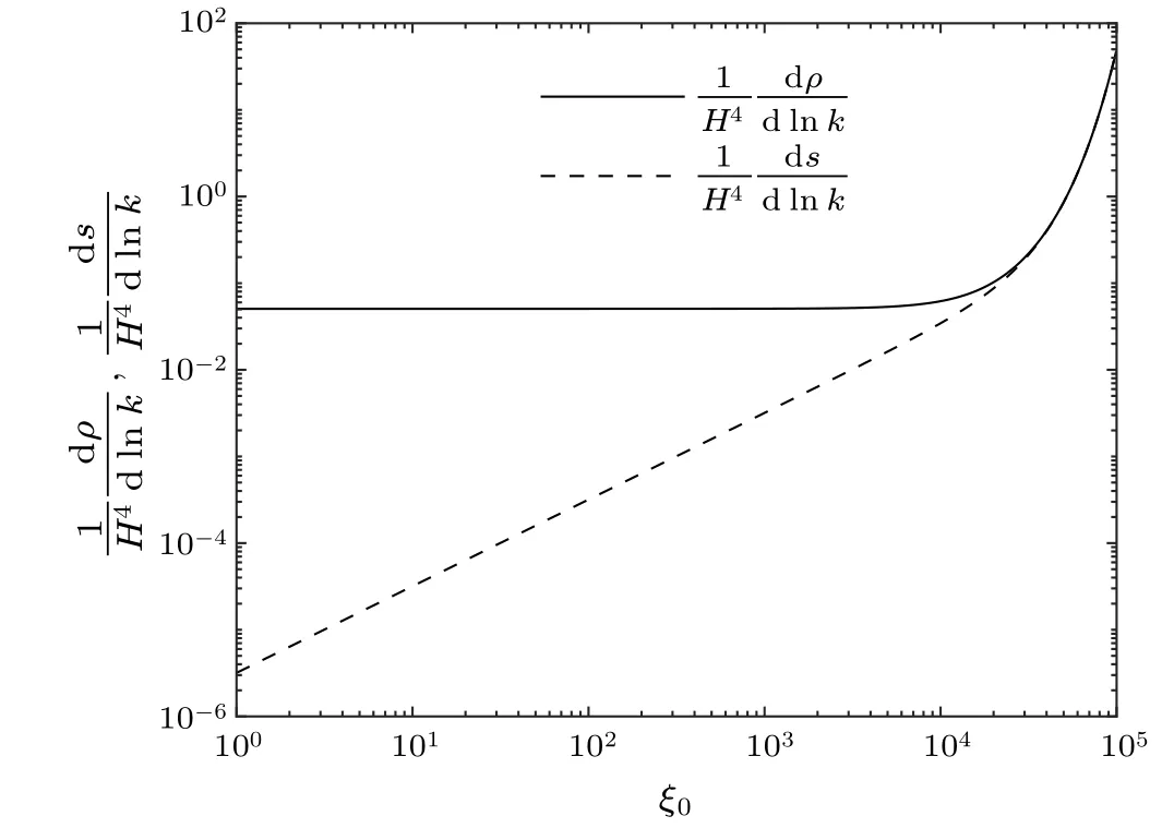
Fig.1.The spectral energy(solid line)and polarized(dash line)density of primordial radiation field to ξ0 by setting k=k*and ε1/2/(1+Q)=10-3.
3.3.Geometrical dynamics vs.thermal dynamics
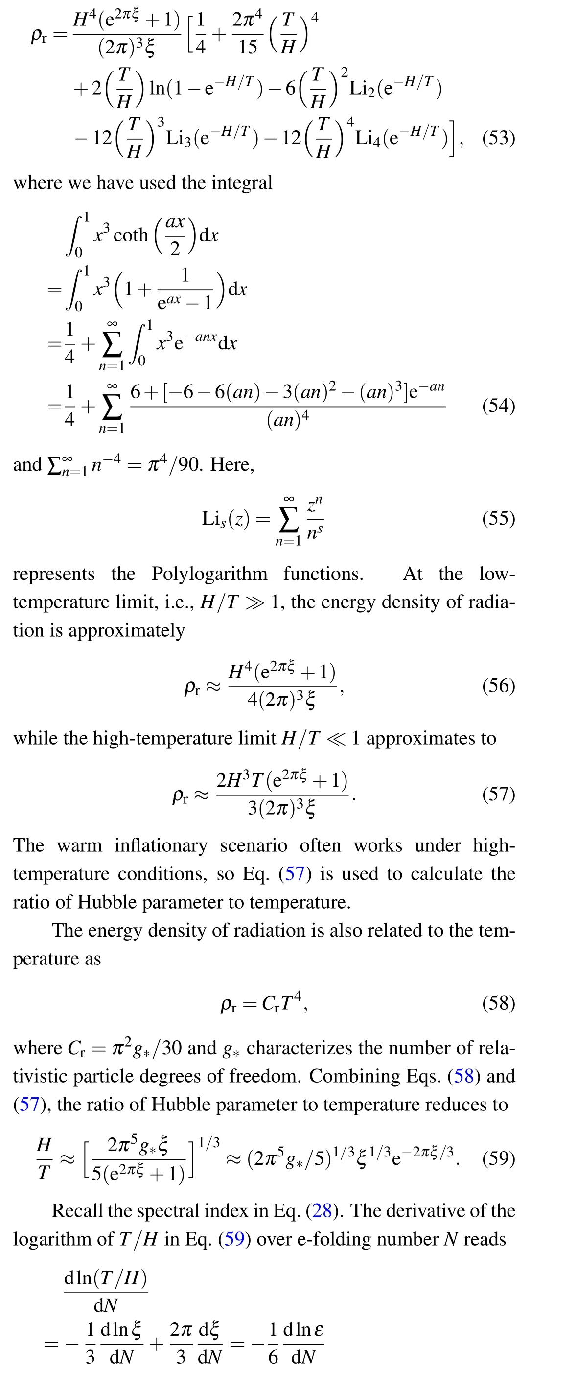
The energy density of radiation is obtained by integrating the spectral energy density:[36]
whereki ~0 denotes the crossing horizon scale at the beginning of inflation.The integral containing the hyperbolic cotangent function is calculated via the series expansion method:
4.Numerical analysis of thermal dynamics
4.1.Dynamical equations and numerical estimation
In the above sections, the discussions do not involve the specific form of natural potential(6).Now we are making further discussions based on this potential.
Introduce the dimensionless variables dN=Hdt,x=φ/f,y=H/Mpandz=H/T.Then, Eqs.(2), (9) and (53)become closed equations
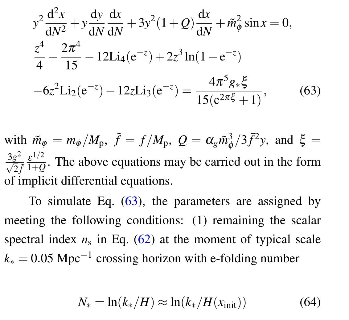
in tune with the current observations;(2)inflation ending with e-folding numberNend≈60 corresponding to the condition in which the slow-roll parameterεHis approximately to unit,i.e.,εH ≈1;and(3)the temperature holding the order at least 109GeV when the Universe entering the radiation-dominate epoch.Moreover, the potential is set asΛ ~10-2Mpto ensure the Hubble expansion rateH ~10-5Mpandg*=106.75.Here the constraint from tensor-to-scalar ratio does not take into account and it will be fully used at the end of this section.

Table 1.Numerical estimation from different combinations of parameters and relevant cosmic quantities based on them.
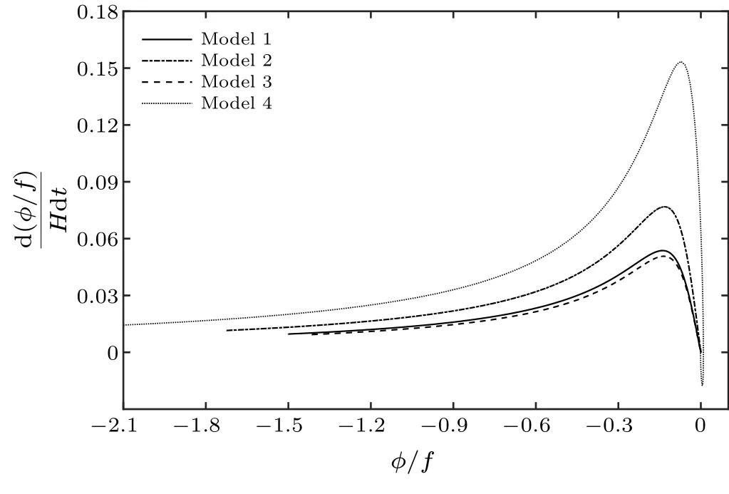
Fig.2.Phase diagram of inflaton mean field φ/f and its velocity of models 1–4 listed in Table 1.
Table 1 lists four typical models satisfying the above three conditions.Model 1–3 are three typical models with strong dissipative coefficients which avoid oscillation at the potential bottom.The dissipative coefficient in model 4 is much smaller, showing an oscillation at the bottom.The phase diagrams of inflaton mean fieldφ/fand its velocityare plotted in Fig.2.Any model introduced above appears a transition from acceleration to deceleration which locates at the epoch between inflation and radiation dominating.
Figure 3 illustrates the temperature evolutions of each model mentioned above.We see that the warm inflation model avoids the reheating process and the temperature decreases gradually, which is a unique physical phenomenon of the warm inflation model.[16,28]It is also found a transition stage between inflationary epoch and radiation-dominate epoch,and the radiation-dominate epoch begins atN ~70.Teqin Table 1 is the temperature at the moment of equality between potential energy and radiation energy.The model with weak dissipative coefficient(model 4)shows a temperature oscillation after inflation when the axion field moves near the potential bottom,corresponding to the oscillation ofφphase diagrams shown in Fig.2.Then, Fig.4 plots the the curves of energy density of different components.It is confirmed that the radiationdominate epoch starts with potentialV(φ)dropping below radiation energyρr, while the kinetic energy ˙φ2/2 remains always subdominant.
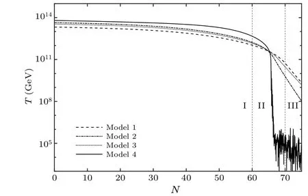
Fig.3.Diagram of temperature T vs e-folding number N with different model.Region I denotes the inflationary epoch, region III denotes the radiation-dominate epoch and II means the transition epoch between them.
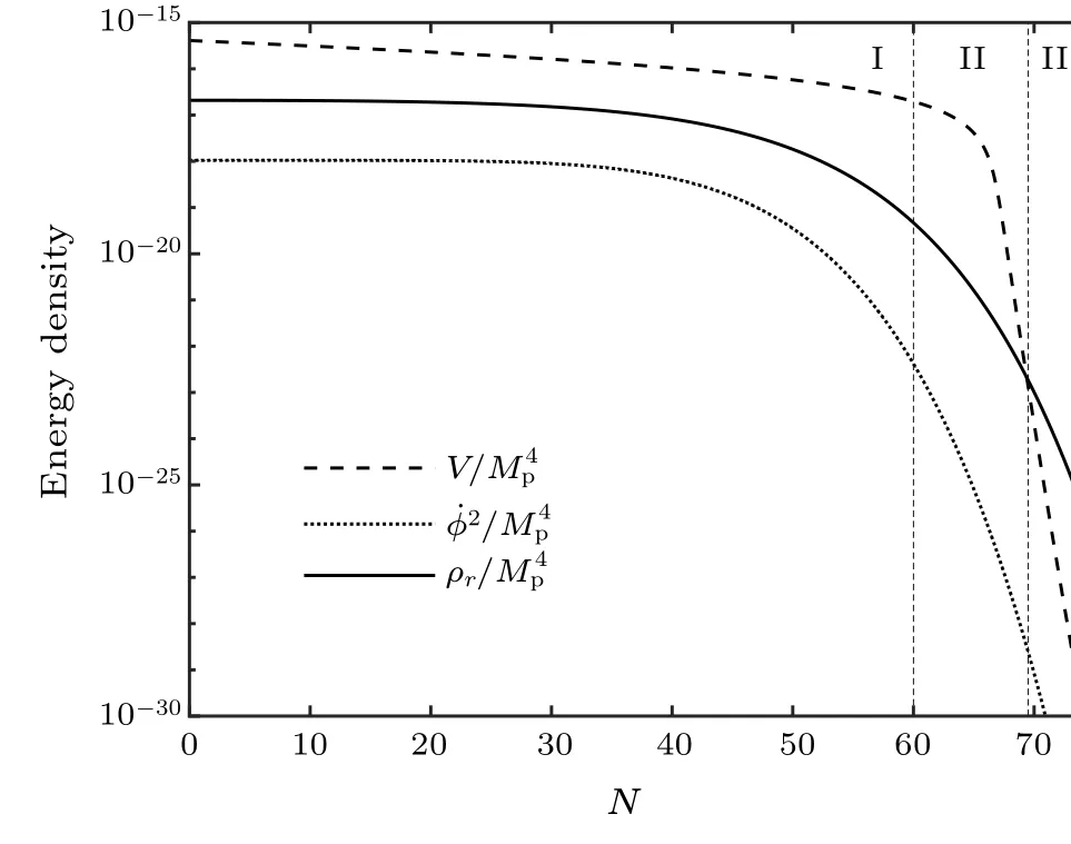
Fig.4.The evolution of the potential,kinetic and radiation energy densities for model 1.The three regions from left to right are inflationary, transitional and radiation-dominate epoch, as the same as those in Fig.3.
4.2.Thermodynamics
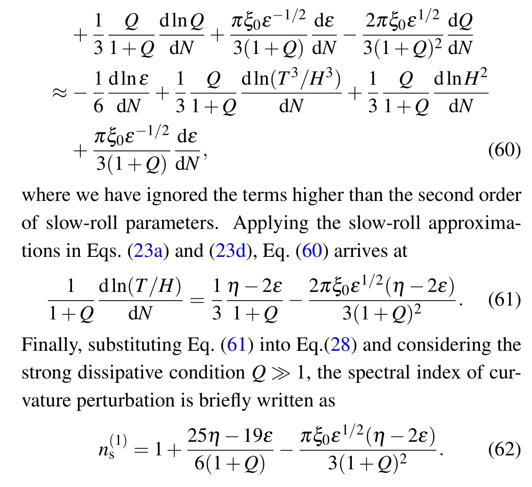
As also seen in Fig.3, the temperature during inflation tends to a constant for any model.This result means that adiabatic approximation still holds in the warm inflationary scenario.Another interesting conclusion is that the coupling constantghas a direct effect on the behavior of temperature during inflation.As it is numerically plotted in Fig.5,the ratioH/Tis not sensitive togif it is less than a specific value.The dataH/Tin Table 1 mean the values in different models.When coupling constantgis less than a threshold,H/Tholds a parameter-independent constant 0.3377.In contrast,a stronger interaction constantgmeans a higher inflationary temperature, since a more intense conversion from vacuum potential to thermal radiation.From this perspective, radiation energy dominates the cosmic evolution whenξ(orε)increases to a critical value.It is also well explained why the temperatures of different model have a slightly difference between each other,as shown in Fig.3.
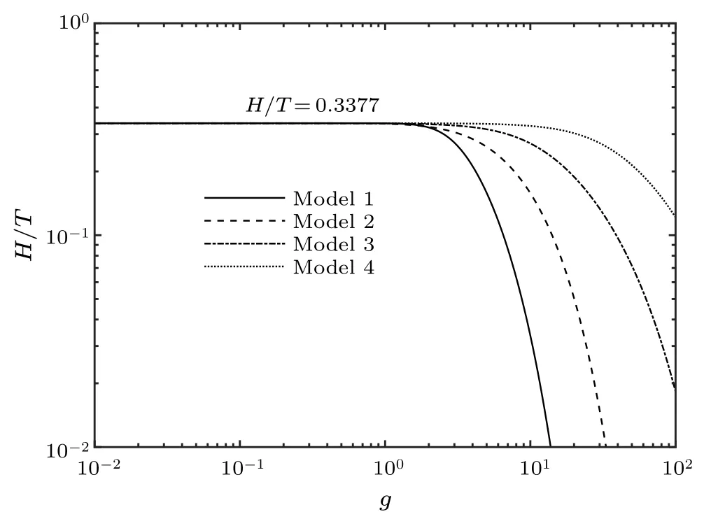
Fig.5.Ratio of Hubble parameter to cosmic temperature H/T in terms of coupling constant g in different models.
4.3.Constrain on the parameters
Equation(63)is the accurate system of equations to simulate the thermal evolution after inflation but not convenient to constrain the relevant parameters.A concise method to constrain the parameters via the observational data is based on the slow-roll approximation.Inflation ends withεH=1,namely,Here,the approximation(11)with? ?3Hand axion-like potential(6)have been used.Thus, the initial value of inflation field is obtained by solving Eq.(68),
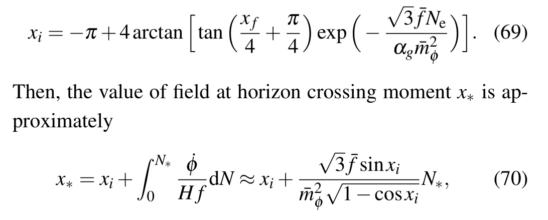
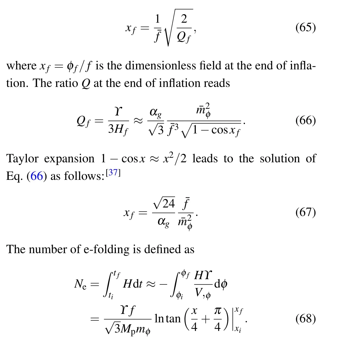
whereN*is introduced in Eq.(64).Substitutingx*into slowroll parametersε,ηandQ,we can finally obtain the value of typical spectral index in Eq.(62).Another observable cosmic parameter we are interest in is the tensor-to-scalar ratior=?2h/?2R, where?2hhas been obtained in Eq.(21) and?2h=2H2/π2M2pis the standard expression of vacuum tensor perturbation.Thus, we have the tensor-to-scalar ratio at typical scale crossing:
The red narrow bands in Fig.6 represent the 95%CL of spectral indexnsfrom the Planck Collaboration data[23]and the orange area in upper half represents the tensor-to-scalar ratiorwithin 95% CL.The dashed lines are contours of ratioH/T.The upper 95% CL band constrains the parameters with larger coupling constant,which means the non-oscillation modes after inflation epoch,as models 1–3 in Table 1.Noticeably, the lower band describes the mode with oscillation at the potential bottom, as seen in model 4.From the results in Fig.6, it can be seen that observational data favors the nonoscillatory models, and the ratio of the Hubble parameter to cosmic temperature is estimated to beH/T ≤0.3377.
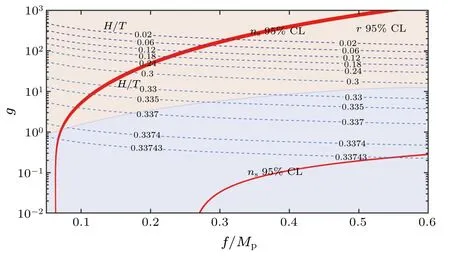
Fig.6.Diagram of spectral index ns and ratio H/T in terms of g and f.The red bands are the 95%CL regions of ns from the observational data, and the dashed lines with specific value are the contours of ratio H/T.Orange area of the upper half-plane represents the 95% confidence region of tensor-to-scalar r.
5.Conclusions and outlook
In this study we introduce the model with inflaton coupling toU(1) gauge field by Chern–Simons interaction and calculate its spectral index under the warm inflationary frame.Regarding the gauge field as a radiation bath, we also calculate the evolutionary trend of the ratio of Hubble parameter to cosmic temperatureH/T.Lastly,numerical method is applied to analyze the relevant parameters or variables during and after inflation.By selecting the appropriate parameter combination,non-oscillating and oscillating phase diagrams are given.We find that cosmic temperatureTtends to a constant during inflation and drops dramatically below the potential energy after inflation, showing a natural transition from inflation to radiation-dominant epoch.The temperature keeps a constant approximately as well during inflation meaning the adiabatic approximation still holding in warm inflation.The ratio of Hubble parameter to cosmic temperatureH/Twill tend to the constant 0.3377 if coupling constant is less than a threshold,being slightly dependent on relevant cosmic parameters.
Research on more complex models will be carried out in the future work.A direct idea is to calculate the spectral law of density and polarized spectrum in the model of non-Abelian axionic inflation and to test whether it can still meet the thermodynamically adiabatic phenomena shown in Figs.3 and 5.Hence, more careful discussions on the thermal effect about warm inflation are necessary.For the rationality of the warm inflation, the conclusions obtained here need to be further verified,such as whether these conclusions can be extended to other models like reheating model with interaction-f2(φ)FμνFμν,whether the warm inflation model can predict the observation effects different from the cold inflation,and so on.Therefore,our next step is to have a detailed discussion on the issues raised above.
Acknowledgments
This work was supported by the National Natural Science Foundation of China (Grant Nos.11864030 and 62061037), Inner Mongolia Natural Science Foundation(Grant Nos.2021LHBS01001 and 2020BS02011), and the Scientific Research Funding Project for Introduced High Level Talents of IMNU(Grant No.2020YJRC001).
- Chinese Physics B的其它文章
- The application of quantum coherence as a resource
- Special breathing structures induced by bright solitons collision in a binary dipolar Bose–Einstein condensates
- Effect of short-term plasticity on working memory
- Directional-to-random transition of cell cluster migration
- Effect of mono-/divalent metal ions on the conductivity characteristics of DNA solutions transferring through a microfluidic channel
- Off-diagonal approach to the exact solution of quantum integrable systems

