Weixi LI() Rui XU()

1.School of Mathematics and Statistics,Wuhan University,Wuhan 430072,China

2.Hubei Key Laboratory of Computational Science,Wuhan University,Wuhan 430072,China

E-mail:wei-xi.li@whu.edu.cn;xurui218@whu.edu.cn

Tong YANG()?

Department of Mathematics,City University of Hong Kong,Hong Kong,China

E-mail:matyang@cityu.edu.hk

Abstract We consider a Prandtl model derived from MHD in the Prandtl-Hartmann regime that has a damping term due to the effect of the Hartmann boundary layer.A global-in-time well-posedness is obtained in the Gevrey function space with the optimal index 2.The proof is based on a cancellation mechanism through some auxiliary functions from the study of the Prandtl equation and an observation about the structure of the loss of one order tangential derivatives through twice operations of the Prandtl operator.

Key words magnetic Prandtl equation;Gevrey function space;global well-posedness;auxiliary functions;loss of derivative

Dedicated to Professor Banghe LI on the occasion of his 80th birthday

1 Introduction and Main Result

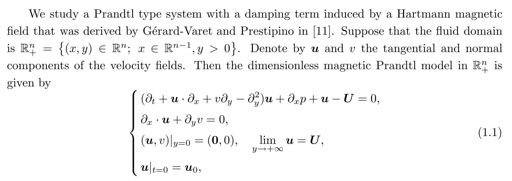
where?xpand U are the traces of a given Euler flow satisfying the Bernoulli law

System(1.1)is derived from the incompressible MHD system in the mixed Prandtl/Hartmann regime,where the leading order equations are

where b stands for the tangential magnetic field satisfying that?yb trends to 0 asy→+∞.By the second equation in(1.2)and the boundary conditions of(u,b),the magnetic fields b can be determined in terms of u;that is,

Then system(1.2)reduces to(1.1).We refer to [11]for the detailed argument.Compared with the classical Prandtl system,there is an extra damping term in(1.1);this does not lead to any additional difficulty in the local-in-time existence and uniqueness theory.Hence,the local well-posedness theories of the classical Prandtl system in Sobolev or Gevrey function spaces established in [2,5,16,28]hold for(1.1).On the other hand,we can expect a global-intime solution to(1.1)because of the damping effect.In fact,some results in this direction were obtained in Xie-Yang [37]and Chen-Ren-Wang-Zhang [3]in the analytic and Sobolev spaces,respectively,about the 2D global stability of the Hartmann layer that satisfies Oleinik’s monotonicity condition.This paper aims to study the global-in-time property of the system for general data without any structural assumption.

Compared with the local-in-time well-posedness theory(see,for instance,[2,4–7,9,12–14,17,20,24,38–41]and references therein),the global-in-timeproperty of the Prandtl system is much less known so that it is far from being well understood.Here we refer to an early work on weak solutions by Xin-Zhang [38],and a work on analytic solutions by Paicu-Zhang [29]and the improvement to Gevrey class 2 by Wang-Wang-Zhang [36].We also mention some other related works [13,39,41].For the Prandtl system with a suitable background magnetic field,the local solutions in Sobolev or Gevrey function spaces were obtained in [19,21,23,25],and the global analytic solution was established recently in [15,26].Note that all of these global-intime existence results are in 2D setting under some suitable structural conditions on the initial data.Hence,the global-in-time properties of these systems in 3D setting remain unknown.

On the other hand,there have been some recent studies on the global well-posedness of hydrostatic Navier-Stokes equations(also called hydrostatic Prandtl equations);these can be used to describe a large scale motion in atmospheric and oceanic sciences,and are derived as a limit of the Navier-Stokes equations in a very thin domain.The hydrostatic Navier-Stokes equations have the same degeneracy structure as in the classical Prandtl system,so that the analytic regularity is sufficient to obtain the local well-posedness theory for general initial data without any structural assumption.Moreover,dueto the damping effect,by combining the vertical diffusion and the Poincar′e inequality in the vertical interval,the global-in-time property of the hydrostatic Navier-Stokes equations was recently verified by Paicu-Zhang-Zhang [31].However,differently from the classical Prandtl equations,the analytic regularity is necessary for the well-posedness theory of the hydrostatic Prandtlequations without any structural assumption(cf.Renardy’s work [32]).Hence,in order to investigate the well-posedness theory in a larger function space than analytic,some structural conditions are required.We mention that the well-posedness in Sobolev space of the hydrostatic Navier-Stokes equations remains unknown.Under the convex assumption,Masmoudi-Wong [27]established the well-posedness in a Sobolev space of the hydrostatic Euler equations which is the inviscid version of the hydrostatic Navier-Stokesequation.However,under the same convex assumption,the well-posedness has been proved for the hydrostatic Navier-Stokes equation only in the Gevrey function space by G′erard-Varet-Masmoudi-Vicol in [10],with the Gevrey index being up to 9/8,and in [8,35]up to 3/2 that is believed to be optimal.Furthermore,the global well-posedness theory of the hyperbolic version of the 2D hydrostatic Navier-Stokes equation was obtained recently by Aarach [1]and Paicu-Zhang [30]in analytic and Gevrey function spaces,respectively,with the extension to the 3D case in [22].A similar well-posedness result on the hyperbolic Prandtl equations in Gevrey class was proven in [18].These results imply that the hyperbolic feature may lead to some kind of stability effect compared with the parabolic counterparts.

This work aims to combine some kind of intrinsic hyperbolic structure with the extra magnetic damping term to derive the global-in-time well-posedness for general Gevrey classes with sharp index 2 initial data without any structural assumption.More precisely,inspired by [5,16],we introduce some auxiliary functions to cancel the nonlocal terms involving the loss of tangential derivatives,and then investigate the intrinsic hyperbolic feature for evolution equations of the auxiliary functions.

In the discussion that follows,we assume that U=0and that?xp=0.We expect the approach can be applied to the case with a more general outer flow satisfying some suitable conditions;that is,we consider system(1.1)as

Note(1.3)is a degenerate parabolic system with a loss of tangential derivatives in the nonlocal normal velocity given by

as the main degeneracy feature of the Prandtl type equations.

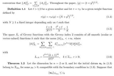
for some sufficiently smallε0>0.Then the magnetic Prandtl model(1.3)admits a unique global solution u∈L∞([0,+∞[;Xρ)with

Remark 1.3Note that the same argument shows that the global well-posednessproperty holds for a Gevrey function space with the Gevrey index in the interval [1,2].

2 A Priori Estimate in 2D

To have a clear presentation,we give a detailed proof of Theorem 1.2 in 2D.Forn=2,we have the scalar tangential velocityu,and then the magnetic Prandtl model(1.3)can be written as

The key part is to derive an a priori estimate for(2.1)so that the existence and uniqueness stated in Theorem 1.2 follows from a standard argument.Hence,for brevity,we only present the proof of the following a priori estimates for solutions to(2.1)with Gevrey regularity:

Theorem 2.1LetXρbe the Gevrey space given in Definition 1.1.Suppose that the initial datumu0in(2.1)belongs toX2ρ0for someρ0>0,and letu∈L∞([0,+∞[;Xρ)be any solution to(2.1)satisfying that

whereρis defined by(1.7).If

for some sufficiently smallε0>0,then

2.1 Method ologies and Auxiliary Functions

The main difficulty for the well-posedness of Prandtl type equations comes from the loss of tangential derivatives.To overcome the tangential degeneracy,the abstract Cauchy-Kowalewski Theorem is an effective method,for example,for the local existence and uniqueness in an analytic setting,cf.[33].However,it is not trivial to relax the analyticity regularity to a larger function space such as Gevrey space for well-posedness.For this,some intrinsic structure of the system needs to be used,cf.[5,16].As was shown in [18,22,30],the well-posedness is well expected in the Gevrey class rather than the analytic setting for the hyperbolic Prandtl equations without any structural assumption.This indicates that the hyperbolic feature may act as a stabilizing factor for the Gevrey well-posedness theory.In this paper,with the extra damping term in magnetic Prandtl model,we will provetheglobal-in-timeexistencein a Gevrey function space by exploring the intrinsic hyperbolic feature for auxiliary functions.

In order to clarify the stability effect of the hyperbolic feature,let us use the following toy model with a hyperbolic factorto illustrate the main idea in the proof:

where one orderx-derivative is lost in twice-time differentiation.Denoting thatg=?th,the above Cauchy problem can be rewritten as

To overcome the loss of thex-derivative,we introduce a decreasing function of radiusρ=ρ(t).In what follows,ρdepends on timet,but we only write it asρinstead ofρ(t)for simplicity of the notations.Moreover,we denote byρ′andρ′′the first and the second time derivatives ofρ,respectively.Now we derive estimates on the Gevrey norm

where(h,g)solves the Cauchy problem(2.5).By direct calculation and using the fact thatρ′≤0,we have that

where l.o.t.refers to the lower-order terms that can be controlled directly.Moreover,we have(cf.Subsection 2.2 for details)that

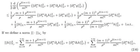
then it follows from the above inequality that

provided that‖h‖L∞is bounded by|max {ρ′,ρ′3}|becauseρ′<0.

Differently from the hyperbolic toy model(2.4),the magnetic Prandtl model is a parabolic initial-boundary problem.If we perform estimates for the 2D magnetic Prandtl model(2.1)directly,the above energy estimate cannot be closed in the Gevrey norm‖·‖Xρ.In order to over come the loss of derivative difficulty,as in [5,16],some an xilliary functionsareneeded.More precisely,for a solutionu∈L∞([0,+∞[;Xρ)to(2.1)satisfying the conditions in Theorem 2.1,let U be a solution to the problem

The existence of U follows from the standard parabolic theory.In fact,one can first apply the existence theory for linear parabolic equations to construct a solutionfto the initial-boundary problem

The above auxiliary functions are slightly different from those introduced in [16]which were inspired by [5].As in [16].by U and

wecan cancel the term involvingvwith the highest tangential derivative as shown in Subsection 2.2.The two auxiliary functions have the relation

In addition,

Recall that the main structure of(2.4)or(2.5)is that the loss of the one orderx-derivative occurs in the twice-time differentiation.If U behaves like the 3-orderx-derivative ofu,then(2.11)–(2.12)admit a similar structure as shown in toy model(2.5).More precisely,we have the loss of one orderx-derivative in the twice application of the Prandtl operator instead of a time differentiation so that the pair(U,?xλ)plays a similar role as(h,g)in(2.5).Inspired by the triple norm defined in(2.6),we define the norms on the solutions and the auxiliary functions as follows:

I held out the chain. She took it in both her hands, reached forward, and secured the simple clasp at the back of my neck. She stepped back then as if to see that all was well. I looked down at the shiny piece of glass and the tarnished13 golden chain, then back at the giver. I meant it when I whispered, Oh, Maria, it is so beautiful. She would have loved it. Neither of us could stop the tears. She stumbled into my arms and we wept together. And for that brief moment I became her mother, for she had given me the greatest gift of all: herself.

Definition 2.2Let U,λbe defined as in(2.7)and(2.10),respectively.By denoting

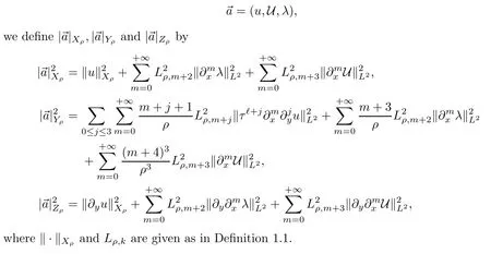
Remark 2.3The norms defined above satisfy that

Ifρ≤1,then

In view of the above remark,the a priori estimate given in Theorem 2.1 holds from the following theorem:

Theorem 2.4Under the same assumption as in Theorem 2.1 we have that

The proof of this theorem is given in Subsections 2.2-2.4.To simplify the notations,we will useCto denote a generic constant which may vary from line to line and depend only on the Sobolev embedding constants and the constants?andρ0in Definition 1.1 and(1.7).Observe thatXr1?Xr2forr1≥r2.Then we can assume,without loss of generality,that the initial radiusρ0≤1.We now list some facts that follow directly from the definition(1.7)ofρ.Fort≥0,

Recall thatLρ,mis defined in(1.6).Then

We will use the following Young’s inequality for discrete convolution:

Here {pj}j≥0and {qj}j≥0are positive sequences.As an immediate consequence of(2.15),

holds for any positive sequences {pj}j≥0,{qj}j≥0and {rj}j≥0.

2.2 Estimate on the Auxiliary Functions

The following proposition is the main part of the proof for Theorem:2.4.

Proposition 2.5Under the same assumption as that in Theorem 2.1,we have that

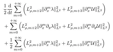
First of all,the auxiliary functionλsatisfies the following equation:

whereHis given in(2.18).

The next lemmas are for the estimate on the last term on the right side of(2.19).

ProofIt suffices to prove the first estimate because the second one can be obtained similarly.

Step 1For simplicity of notation,set

We first prove the following two estimates for L(u,U):

In fact,Leibniz’s formula gives that

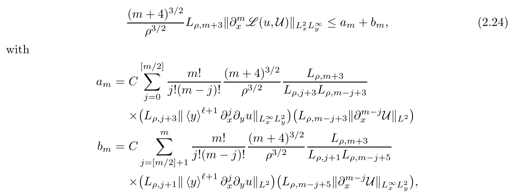
where [m/2]represents the largest integer less than or equal tom/2.Direct computation shows that,for any 0≤j≤[m/2],

where we have used the fact thatρ0/2≤ρ≤ρ0in the last inequality.Then

where we have used Young’s inequality(2.15)for discrete convolution.Similarly,by using the estimate

Combining the above estimates with(2.24)yields(2.22).

Step 2To prove(2.20),Leibniz’s formula gives that

Straightforward calculation shows that

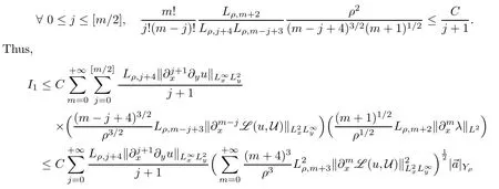
where we have used(2.16)in the second inequality and(2.22)in the last inequality.

ForI2,by(2.23)and the estimate

we have that

Substituting the above estimates onI1andI2into(2.25)yields the first estimate of(2.20)in Lemma 2.6.

Step 3It remains to prove the second estimate in Lemma 2.6.For this,write

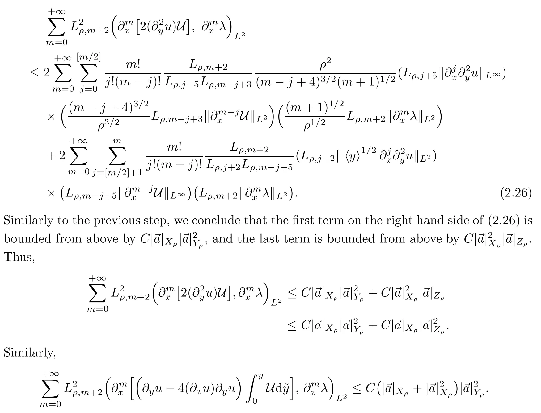
Combining the above two estimates gives the second estimate in Lemma 2.6.This completes the proof of the lemma. □

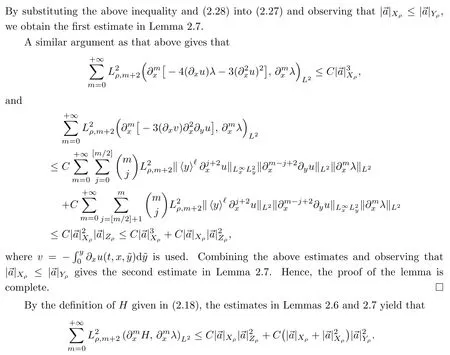
Therefore,we have,by the equality(2.19),the following corollary:

Corollary 2.8(Estimate forλ)Under the same assumption as in Theorem 2.1,we have that

We now turn to derive the estimate on U.

Lemma 2.9(Estimate on U)Under the same assumption as in Theorem 2.1,we have

ProofBy(2.9)and the boundary condition that?yU|y=0=U|y=+∞=0,the energy estimate on(2.11)gives

Note that the first term on the right side is non-positive and the second one is bounded from above by

For the last term in the above inequality,a similar argument as that for Lemmas 2.6 and 2.7 yields that

Combining the above estimates completes the proof of the lemma. □

Proof of Proposition 2.5Combining the estimates in Corollary 2.8 and Lemma 2.9 gives that

where we have used the fact thatρ′/2≤ρ′3/2≤ρ′3/4 in the last inequality.

It remains to estimate the first term on the right hand side of(2.29)as follows:

Then,Proposition 2.5 follows by combining(2.29)and(2.30).

To prove(2.30),denote that

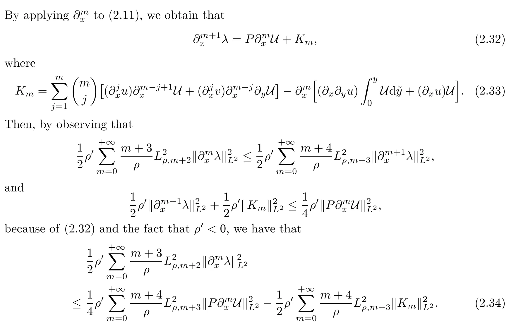
The two terms on the right hand side of the above inequality will be estimated as follows:

(i)Estimate on the last term on the right hand sid e of(2.34).Noting that?ρ′/ρ≤1,by the defintion ofKmin(2.33),we have that

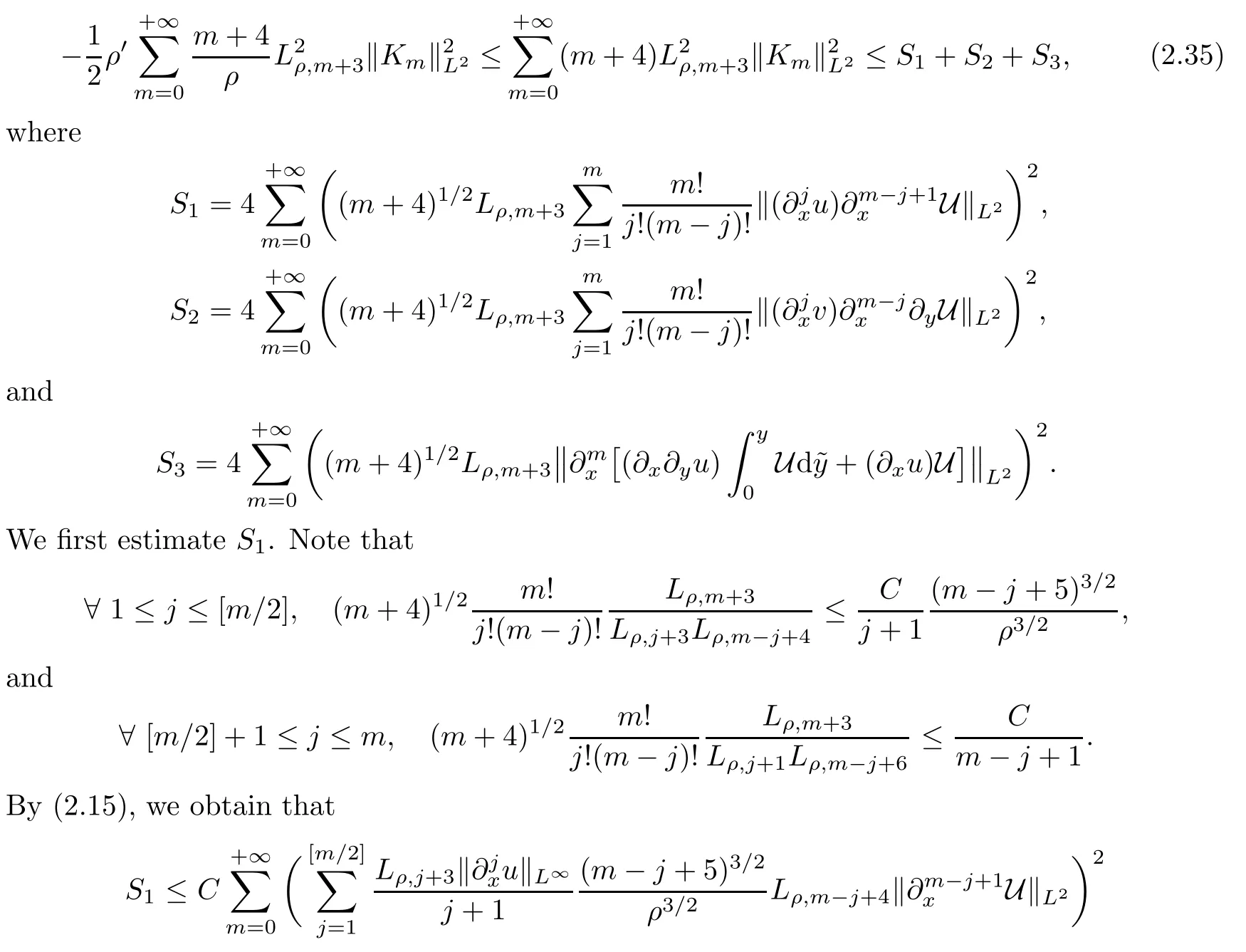
Substituting the above estimate and(2.36)into(2.34)yields(2.30).Thus,the proof of proposition is complete. □

2.3 Estimate on the Tangential Velocity

We now derive the estimate on‖u‖Xρ.

Proposition 2.10Under the same assumption as in Theorem 2.1,the estimate

holds for any 0≤k≤3,whereτis defined as in(1.4).

ProofWe will basically give the estimates in the cases of whenk=0 andk=3.

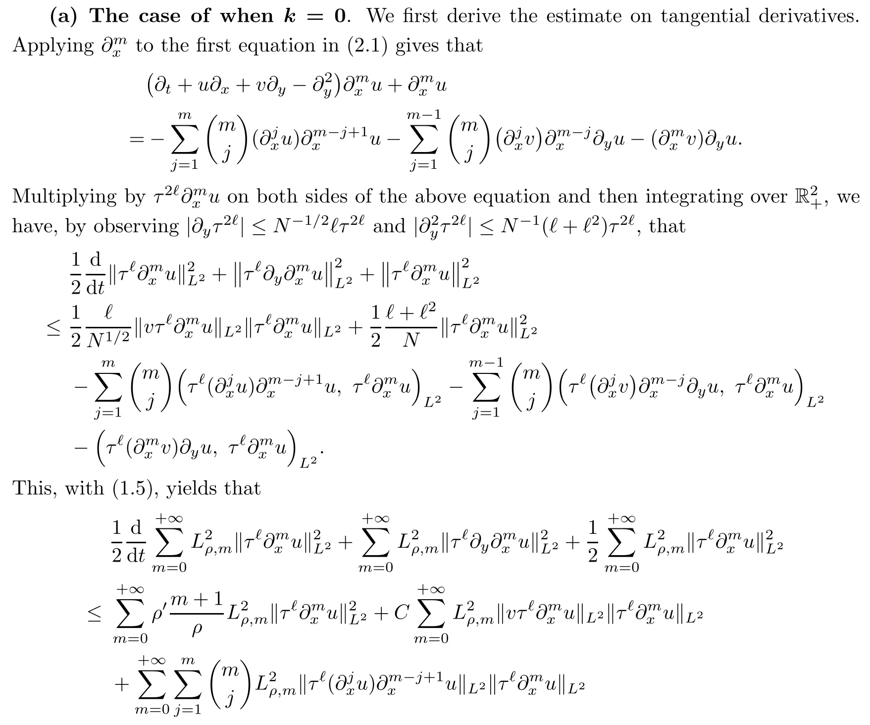
Direct calculation gives that

Similarly to the proofs of Lemmas 2.6 and 2.7,we have that

It remains to estimate the last term in(2.37).Direct calculation gives that

Form≥2,by recalling L(u,U)given in(2.21),we use(2.10)to write that

Thus,

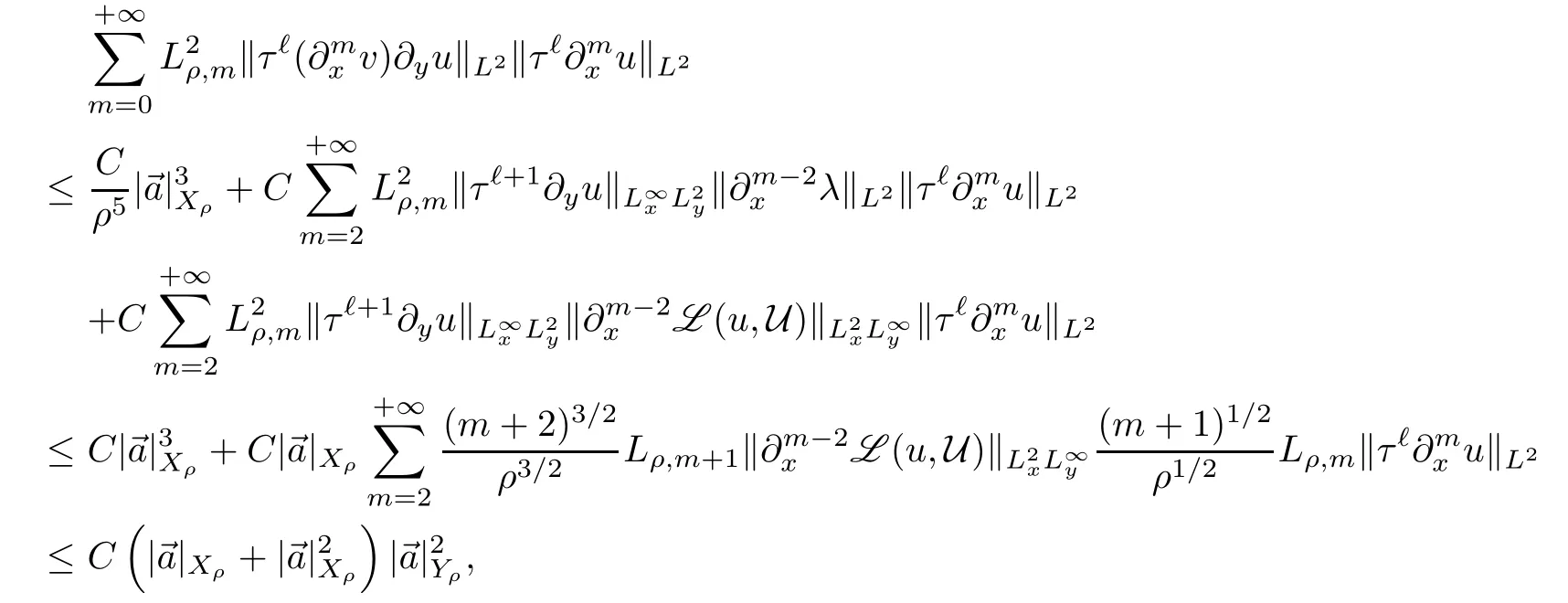
where we have used(2.22)in the last inequality.By substituting the above estimates and(2.38)–(2.39)into(2.37),and by using the fact thatρ′≤ρ′3≤ρ′3/4≤0,we have that

Thus,Proposition 2.10 holds fork=0.

The assumption(2.2)implies that each term in the above equation belongs to

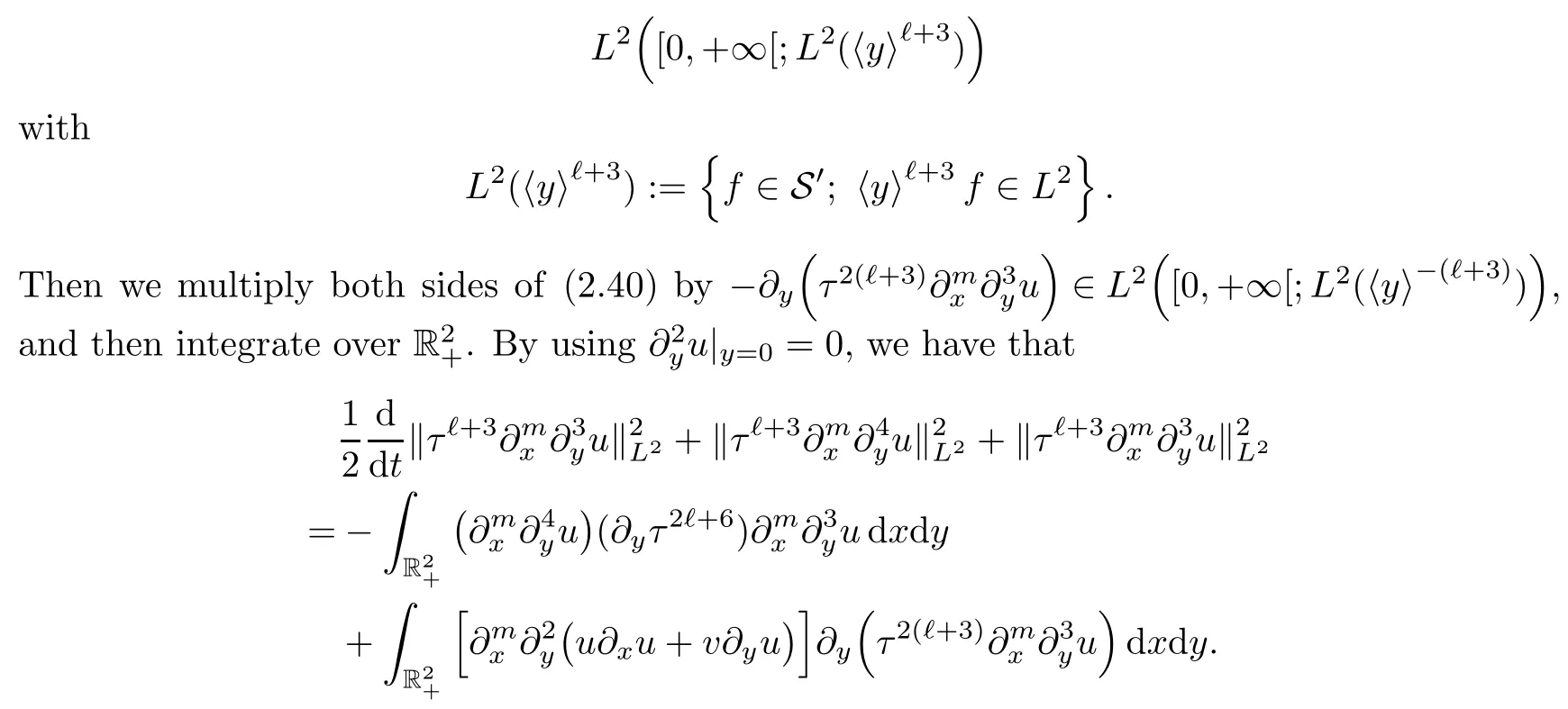
For the terms on the right hand side of the above equality,we have that

This proves Proposition 2.10 fork=3.

The cases of whenk=1,2 can discussed similarly,so we omit the details,for brevity.The proof of proposition is complete. □

2.4 A Priori Estimate in 2D

Wewill apply the following abstract version of the bootstrap principle given in [34]to prove Theorem 2.4:

Proposition 2.11(Proposition 1.21 of [34])LettingIbe a time interval,and for eacht∈Iwe have two statements:a“hypothesis”H(t)and a“conclusion”C(t).Suppose that we can verify the following four statements:

(i)If H(t)is true for some timet∈I,then C(t)is also true for the timet.

(ii)If C(t)is true for somet∈I,then H(t′)holds for allt′in a neighborhood oft.

(iii)Ift1,t2,···is a sequence of times inIwhich convergesto another timet∈Iand C(tn)is true for alltn,then C(t)is true.

(iv)H(t)is true for at least one timet∈I.Then C(t)is true for allt∈I.

For eachT∈[0,+∞[,let H(T)be the statement

and let C(T)be the statement

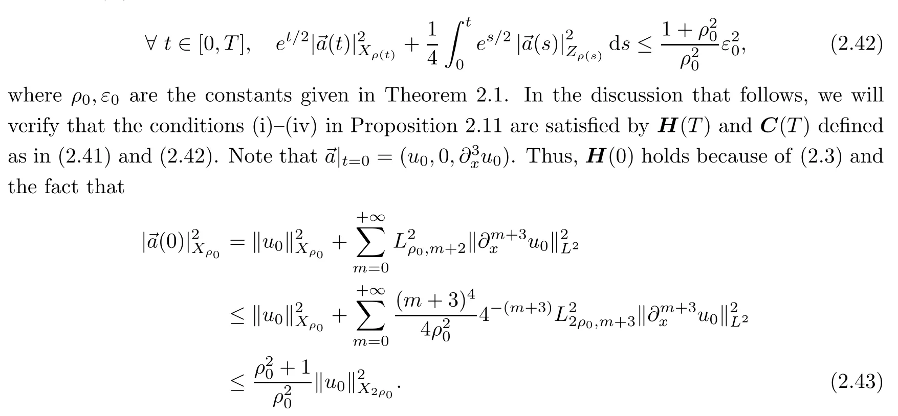
Hence,the condition(iv)in Proposition 2.11 holds.Moreover,the conditions(ii)-(iii)follow from the continuity of the function

It remains to check the condition(i)in Proposition 2.11;that is that

H(T)is true for some timeT>0=?C(T)is also true for the same timeT.

By Definition 2.2,we combine the estimates given in Propositions 2.5 and 2.10 to get that

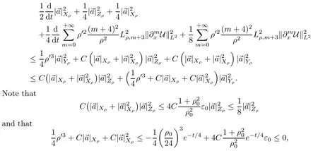
providedε0is sufficiently small.Combining the above estimates implies that

By integrating the above estimate over [0,t]for anyt∈[0,T]and using U|t=0=0,we obtain that

where we have used(2.43).This yields(2.42)if(2.41)holds,so that the condition(i)holds.Therefore,by Proposition 2.11,the estimate(2.42)holds for anyT≥0,and the proof of Theorem 2.4 is complete.

3 A Priori Estimate in 3D

The discussion on the 3D magnetic Prandtl model is similar to that of the 2D case.For this,we will use vector-valued auxiliary functions instead of the scalar ones used in the previous section.More precisely,denote by u=(u1,u2)andvthe tangential and normal velocities,respectively,and by(x,y)the spatial variables in R2×R+withx=(x1,x2).As the counterparts of U andλdefined by(2.7)and(2.10),we define U=(U1,U2)andλ=(λ1,λ2,λ3,λ4)as follows:let Uj,j=1,2,solve the initial-boundary problem

Accordingly,set

The proof of Theorem 3.1 is the same as that of the 2D case,so,for brevity,we omit the details.