Dattaprasad Torse, Veena Desai, Rajashri Khanai

1Department of Electronics and Communication Engineering, KLS Gogte Institute of Technology, Belagavi, Karnataka 590008, India;2Department of Electronics and Communication Engineering, KLE Dr. M. S. Sheshgiri College of Engineering and Technology, Belagavi, Karnataka 590008, India.

Abstract The detection of seizure onset and events using electroencephalogram (EEG) signals are important tasks in epilepsy research. The literature available on seizure detection has discussed the implementation of advanced signal processing algorithms using tools accessed over the cloud. However, seizure monitoring application needs near sensor processing due to privacy and latency issues. In this paper, a real time seizure detection system has been implemented using an embedded system. The proposed system is based on ensemble empirical mode decomposition (EEMD) and tunable-Q wavelet transform (TQWT) algorithms. The analysis and classification of non-stationary EEG signals require the wavelet transform with high Q-factor. However, direct use of TQWT increases the computational complexity of feature extraction from multivariate EEG signals. In this paper, the first step is to process the signal by using EEMD to obtain 8 intrinsic mode functions (IMFs). The Kraskov (KraEn),sample (SampEn), and permutation (PermEn) entropy features of IMFs are extracted and based on optimum values, and 4 IMFs are decomposed using TQWT. Secondly, centered correntropy (CenCorrEn) features of the 1st and 16th sub-band of TQWT have been used as classifier inputs. The performance of multilayer perceptron neural networks (MLPNN), least squares support vector machine (LSSVM), and random forest (RF) classifiers has been tested on the multichannel EEG data recorded from a local hospital. The RF classifier has produced the highest accuracy of 96.2% in classifying the signals. The proposed scheme has been employed in developing an embedded seizure detection system to assist neurologists in making seizure diagnostic decisions.

Keywords: seizure detection, electroencephalogram, ensemble empirical mode decomposition, intrinsic mode function, tunable-Q wavelet transform

Introduction

Epilepsy is caused by irregular changes in neural activity[1]. The recurrent impulsive seizure from intricate processes is related to numerous neurotransmitters in the cholinergic, glutamatergic and GABAergic system[2]. As the World Health Organization reports[3], out of 450 million people worldwide with neurological or behavioral disorders,65 million are affected by epilepsy with nearly 7 million cases in India[4]. The medical diagnosis of epileptic disorders is made by medical professionals using EEG signals recorded from the patient's scalp[5].The two major types of EEG signals are focal and non-focal in generalized epilepsy. The focal EEG signals may be categorized as epileptic or nonepileptic. Epileptic spikes are the interictal indication of a patient with involvement of limited area of the brain. Non-epileptic deformities are characterized by variations in normal signals or by the manifestation of abnormal signals. While these two types often coexist,separating them is conceptually useful and helps in diagnosis of focal epilepsy[6]. The major treatment option for epilepsy is anti-epileptic drugs (AEDs). The best possible AEDs fail to control seizures in practically one-third of epileptic patients and seizures persist for lifetime. The design and development of automated seizure detection systems may have the potential to improve the diagnostic accuracy when compared to manual observations of EEG signals. The signal feature computation and then classification are major steps in computerized seizure detection[7]. EEG signals are a powerful tool in different clinical applications for diagnosis of brain disorders. The computational complexity of signal processing algorithms is a prime factor in real time seizure detection systems[8].

Recently, several automated EEG classification algorithms based on empirical mode decomposition(EMD) and tunable-Q wavelet transform (TQWT) are proposed on single-channel univariate signals for 2-class and 3-class problems. Hassan ARet alhave proposed an automated epilepsy diagnosis scheme based on TQWT and bootstrap aggregating, which reveals applicability of spectral features in the TQWT domain in combination with bagging[9]. Based on statistical moment based features extracted using EMD, sleep scoring on single channel EEG classification using adaptive boosting and decision trees has been presented by Hassan ARet al[10]. A study on use of normal inverse Gaussian (NIG) pdf modeling of TQWT sub-bands in sleep stage classification has been presented by Hassan ARet al[11]. An automated sleep staging method has been developed by Hassan ARet alby using TQWT and different spectral features obtained from TQWT subbands. The classification has been performed by random forest (RF) classifier[12]. Hassan ARet alhave shown the efficacy of automated EEG signal processing systems using TQWT and EMD[13–16].

As in the above literature, the EEG signals are classified using statistical and entropy features. The decomposition of EEG signal and computation of features is done separately in two steps, using either ensemble EMD (EEMD) or TQWT. The single stage decomposition used earlier shows increased computational complexity of the classifiers due to the inclusion of single level decomposition and features.The main advantage of EEMD is in identifying statistical characteristics of white noise when deciding the final number of IMFs. TQWT has an advantage of operating on small/no oscillatory signals with a low Q-factor, but not on high oscillatory signals with a relatively high Q-factor. TQWT handles the issue by adjusting its Q-factor and hence may be used as an effective algorithm for EEG signal analysis. In this paper, advantages of EEMD and TQWT are combined to extract optimum features in two stages to enhance the classification accuracy in a real time seizure detection system.

The proposed joint EEMD-TQWT is shown inFig. 1.In the first step, the EEG signals from normal and seizure classes are decomposed using EEMD. Since the maximum oscillatory information about the signals lies in the first few IMFs, four initial IMFs are selected for decomposition using TQWT based on optimum values of Kraskov entropy (KraEn),permutation entropy (PermEn), and sample entropy(SampEn). The sub-bands of the signals are obtained by choosing low-Qvalues for IMFs with low oscillatory behavior, and high-Qvalues for more oscillatory IMFs. In the second step, experimental results show that the centered correntropy(CenCorrEn) features computed only for the 1stand 16thsub-bands of the selected IMFs results in the highest classification accuracy. The first sub-band of TQWT represents high-pass sub-band and the last low-pass sub-band. Since we have considered 4 IMFs from the EEMD step, a total of 16 sub-bands are produced by the TQWT step. The features from these sub-bands represent oscillatory behavior of decomposed signals. Moreover, with the higher order of sub-band, a reasonably good resolution can be attained concurrently in high and low frequency region of the input signals. The selection of optimum features from this set is done using the wrapper method of feature selection[17]. Finally, a comparison of the classification performance is presented for LSSVM and RF classifiers.

Materials and methods

Electroencephalogram (EEG) dataset

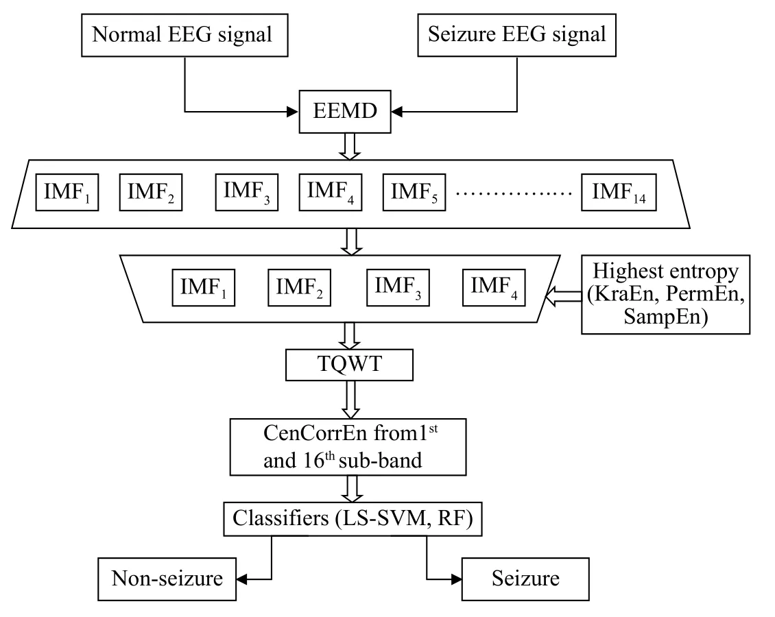
Fig. 1 Joint EEMD-TQWT based system for seizure classification.

This research work used two datasets, namely public and local. The public dataset (http://www.dtic.upf.edu/~ralph/sc/) contains multichannel intracranial EEG records of 5 patients who were suffering from pharmacoresistant temporal lobe epilepsy. Each EEG signal was sampled with 512 Hz sampling frequency and contained 10 240 samples. The band-pass filter of frequency range between 0.5 to 150 Hz has been used to filter noises[18]. In this dataset, 3 750 files were belonging to each class, focal and non-focal and 80%of the dataset have been used to train the machine learning algorithm and test its performance of local dataset. The local dataset contained the EEG data recorded from 10 subjects. The feature extraction and classification algorithms always performed exceedingly well for the online datasets. However, the performance of the same system considerably deteriorated when tested on the real time data recorded from patients. The reason for the adverse performance is unbalanced data resulting from the recording and sampling process in real time. In this work, all four entropy values were computed for multiple channels(19-channels) related to both EEG datasets for detection of seizure activity. The dataset contained 5 healthy subjects' EEG (3 male and 2 female), few with history of chronic headache and none with symptoms of epileptic seizures, and 5 epileptic subjects (3 male and 2 female), aged between 10 to 35 years. The extracranial recording was done with eyes open and closed using standard 10 -20 electrode placement. Out of 5 epileptic subjects, only one child subject of age 12 years was recorded with drug induced sleep EEG.The recording was done for 10-to-15-minutes sessions. The expert neurologist was consulted to read the EEG data manually and decide epileptic seizures identified from the specific channel of the recording system. The system used was Recorders & Medicare Systems (RMS) medical equipment data acquisition 10-20 standard, which enabled recording of EEG from 19 active unipolar channels (FP1, FP2, F7, F3, Fz, F4,F8, T3, C3, CZ, C4, T4, T5, P3, PZ, P4, T6, O1, and O2) with A1 and A2 as a reference connected to total 21 electrodes placed on the subject's left and right head. To maintain uniformity in data samples taken from public and local dataset, selection of 19 channels was done based on comparison with public dataset.An electrode fixed in the middle of distance between FP1 and FP2 on the subject's forehead was the ground.For this pilot research work, time series of approximately 23 seconds (4 000 samples) from the EEG recording was selected for 5 healthy and 5 epileptic patients under the expert observation of the neurologist as shown inFig. 2. The total number of samples was 176/second and hence the EEG data was sampled at 176 Hz. From the recording of original datasets and manual observation, only artifact-free EEG signals were segmented from large datasets.

Ensemble empirical mode decomposition (EEMD)and tunable-Q wavelet transform (TQWT)

In time-scale domain, the sparsity of IMFs obtained from EEMD can be best represented by decomposing them using TQWT. The novel technique of application of TQWT to the IMFs to characterize the oscillatory behavior of EEG was used on F and NF signals. The assessment and selection of IMFs were based on the optimum values of Kraskov, sample and permutation entropies.

Ensemble empirical mode decomposition (EEMD)

EMD is an adaptive joint time-frequency data analysis scheme[18]. The methods work on the principle of decomposing the EEG signal into a finite set of oscillatory elements called intrinsic mode functions (IMFs). The IMFs are considered as zeromean, amplitude and frequency modulated (AM-FM)components. To obtain the correct form of IMF, it should satisfy two conditions[18]: (1) In the complete dataset, the total number of extrema values and the number of zero-crossings have to be either equal or vary at most by one; (2) The mean of two envelopes,one defined by connecting local maxima and the other by local minima, at any point should be zero.

In EMD the original signalx(t) is expressed as

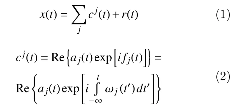
wherecj(t) indicates IMFs andr(t) is the residual non-oscillating signal. Theaj(t) denotes a timedependent amplitude,represents a timedependent phase.

Although the data adaptive EMD is a powerful method to decompose nonlinear signal, it has the disadvantage of the frequent emergence of mode integration. This indicates a mode mixing problem,where a single IMF either consists of signals of widely dissimilar scales, or a signal of a scale alike existing in unlike IMFs. An improved technique of a noiseassisted data analysis (NADA), known as the EEMD,was suggested to eliminate this drawback[19].

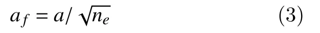
In EEMD, an ensemble of data sets was generated by adding uniformly distributed white noise with finite amplitude 'a' to the original signalx(t). The EMD analysis was then used to each of the data series of the ensemble. Finally, the IMFs were obtained by averaging the individual components in every realization over the ensemble. In EEMD algorithm various parameters such as ensemble number (ne),number of siftings (ns), amplitude of white noise (a),number of IMFs (nimf) and IMF (cm) were defined based on the time complexity of the signal being decomposed. The algorithm was initialized by setting the IMF value [cm(t)]equal to zero. The resulting signal decomposed into IMFs and the trial loop was executed for the maximum value ofne. Finally, the ensemble mean of the computed IMFs from the decompositions was given by[20]

In this work, decomposition of bivariate EEG signal was done by adding optimum values of white noise of amplitude 0.4 and number of ensembles was equal to 10 based on the experimentation performed on both datasets. The IMFs extracted from sample non-focal and focal EEG channel difference signals using EEMD technique were depicted inFig. 3–4.

Tunable-Q wavelet transform (TQWT)

The tunableQ-factor is a prime quality of TQWT that makes it most suited for transform in analysis of IMFs with varying oscillatory nature. Ideally, the ratio of center frequency of an oscillatory signal to its bandwidth, defined as theQ-factor of a wavelet transform should be selected based on the oscillatory frequency components in the signals[14]. However,fixed value ofQ-factor poses limitation on decomposition of nonlinear IMFs. The analysis of high oscillatory IMFs should be done using large value ofQwhereas less oscillatory IMFs need smaller values ofQ. The TQWT is bound by theQ-factor and its redundancy. In decomposing selected IMFs, the TQWT parameters defined are theQ-factor (Q), total over-sampling (r), and the number of decomposition phases termed as (j). The number of oscillations of the wavelet is determined by theQparameter, which has the property of tuning in terms of α and β.

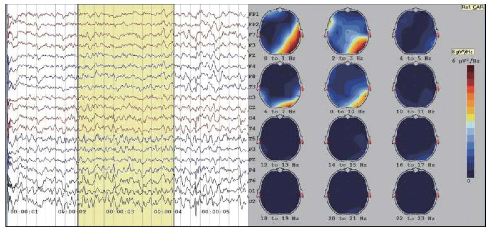
Fig. 2 Amplitude plot and frequency maps of normal EEG dataset of subject for FP1 to O2 channels.

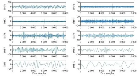
Fig. 3 Intrinsic mode functions from difference of sample 2-channel non-focal EEG signal.

The parametersrandQ-factor forjdecomposition levels is defined as[14]

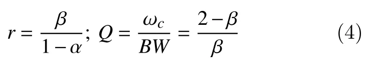
The termBWis bandwidth of the frequency response resulting in 'j' sub-bands.

The selection ofQ-factor and 'r' depend on the number of levels of decomposition to cover the IMF's frequency range. The filter bank parameters α and β are selected to achieve the desired values. For a constant value ofQ, as 'r' increases, overlapping between neighboring frequency responses increase.TQWT filters are easier to implement since the construction of these filters are based on non-rational transfer functions.

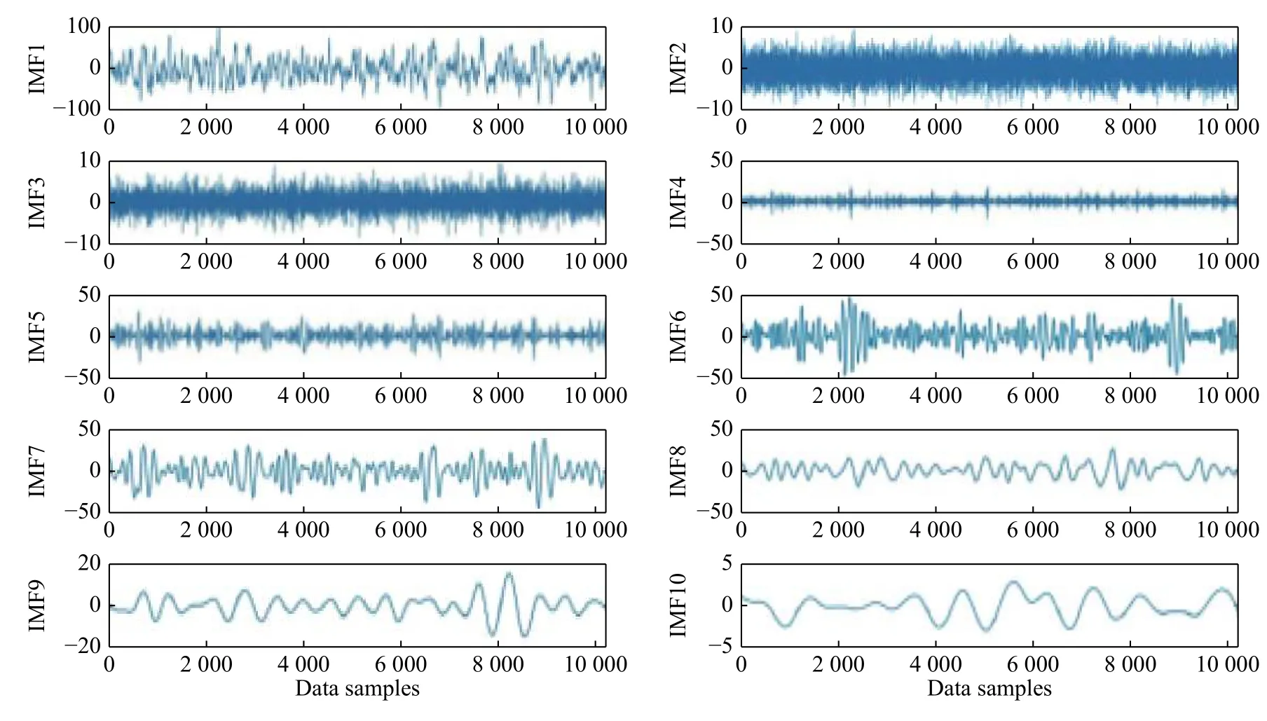
Fig. 4 Intrinsic mode functions from difference of sample 2-channel focal EEG signal.

The multi-stage TQWT decomposition of IMFs can be achieved by repeatable connection of 2-band filter banks to its low pass channel. A 'j-level' TQWT is depicted inFig. 5.

At each level of decomposition, the input signalx(n) is converted into low-pass and high-pass signal components. For the input signal sampling ratefs, the resulting low-pass and high-pass sampling frequencies areαfsandβfswhereαandβare the same scaling constants for all levels of decompositions. The lowpass and high-pass sub-bands are computed using their respective frequency responses and scaling factors. The low-pass and high-pass frequency response factors are determined as shown in equations[14]

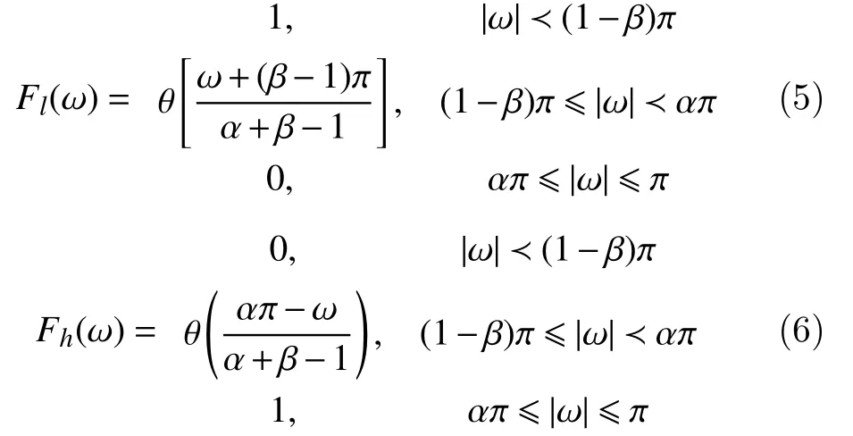
whereθ(ω)is expressed as[13]

Finally, the reconstruction of original input signal is accomplished by using the same filter banks used in the decomposition stage.

Entropy based feature estimation

Normally, classification of seizure and non-seizure EEG signals is achieved using a set of diagnostic features extracted from the signal components. The optimum feature sets with intra-class identical characteristics and inter-class fluctuations are well suited for automated systems. However, proper selection of feature sets and their discrimination ability depends on signal decomposition stage. The entropy features, developed by Shannon are a measure of spread of the data. The entropy is used to quantify unpredictability within the signal and to measure complexity of nonlinear signals. Acharya, U.Rajendra, et al. have proposed a review on applications of entropies in automated diagnosis of epilepsy[21].

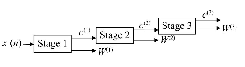
Fig. 5 Two channel analysis TQWT filter bank.

Kraskov entropy (KraEn)

The entropy measure is useful in analyzing nonstationary and nonlinear EEG signals. The Shannon's entropy for a data sourceSis defined using

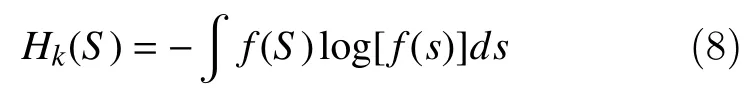
wheref(S) is probability density function (pdf). The differential statistical entropy of nonlinear signals known as the Shannon entropy is measured using KraEn. In this work, KraEn is computed for the EEG signals using the "k-nearest neighbor" sample. By default the Euclidean distance has been used for estimatingH(S) from EEG signals of 'n' samples of signal 'S'. Equation 8 is considered as an average of logμ(Si). For unbiased estimator equation 8 is defined as

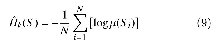
To obtain the estimate ( logμ(Si)), we consider the probability distributionPi(ε)for the distance betweenSiand itskthnearest neighbor. For Euclidian norm, the final entropy is given by

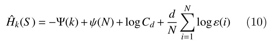
wheredis the length of sourceS,Cdis volume of thed, ψ (N)? ψ(k) is the expected value of the data source, is twice the distance fromSito itskthneighbor[22].

Permutation entropy (PermEn)

By combining the concept of entropy and symbolic dynamics, Bandt and Pompe introduced a new concept of PermEn as a measure of complexity of nonlinear signals by[23]

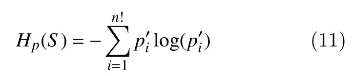
The PermEn per symbol is as given by

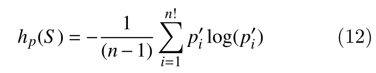
where 0 ?hp(S)?1.

The PermEn is computed with permutation order 'n'using a method which considers the first occurrence order[23].

Sample entropy (SampEn)

SampEn devised by Richman and Moorman[24], is defined as measure of the unpredictability of thei.e.how much a given data point depends on the values ofkof previous data points, averaged over the entire signal range. It is also a measure of data regularity like approximate entropy. SampEn is mostly independent of record length. The detection irregularity in the EEG data is associated to larger values of SampEn.

The SampEn is computed by finding points that are matching within the tolerance 'r' for all match points,whereas the number of template matches are stored in countersA(dim) andB(dim) for all lengthsdimup to'e'. SampEn is defined by

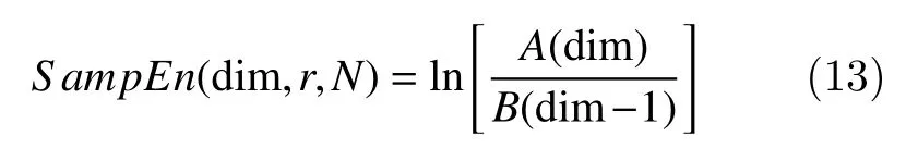
whereB(0) =N, the length of the input series anddimis the embedding dimension andris the tolerance value. The false nearest neighbor has been used in this work to extract SampEn. With the appropriatekvalue the false neighbor value reaches zero. In this work,k=2 was appropriate value for SampEn computation of IMFs[24].

Centered correntropy (CenCorrEn)

In a specific window controlled by the kernel dimension, correntropy straightly specifies the probability density of closeness of two random variables[25]. Cross-correlation is the similarity between two different signals in time domain and its entropy known as correntropy. It is a similarity measure of multichannel signals resulting in nonlinearity of a feature space. The correntropy is defined by

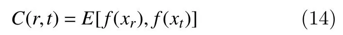
where ? maps nonlinearity between samples from the input to the feature space. Correntropy uses the'kernel trick' that gives the inner product of nonlinear combinations called as Mercer kernel and is defined by

This kernel-trick method results in relevant feature space without the precise knowledge of nonlinear mapping and hence reduces the expected value of the kernel of a particular choice. The most commonly used Mercer kernel is in the form of Gaussian kernel denoted by

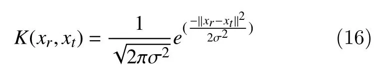
where σ is the size of the kernel.

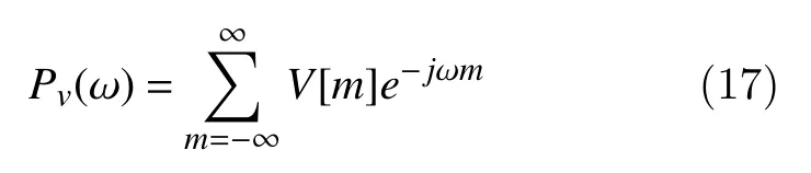
The Fourier transform of correntropy has been introduced as the general power spectral density and defined as correntropy spectral density (CSD)[25]. The CSD is defined by

Classification techniques

In machine learning and statistics, classification deals with identifying a set of class to which a data sample belongs in the sample database. In this work,EEG signal is classified into seizure and non-seizure class. An illustration of supervised learning has considered where training data set of correctly classified samples is available for assessing performance of three classifiers.

Multi layer perceptron neural networks (MLPNN)classifier

Multilayer feed-forward neural networks(MFNN)[26]designed for the problem uses multiple neurons interconnected in basic format of input layer,multiple hidden layers, and an output layer. The basic functionality of multilayer neural networks is the same as that of a traditional one-hidden-layer neural network[26]. In the proposed study, four features were used to train the MLPNN and its performance was eevaluated. The training and testing the MLPNN algorithm begins with configuring the neural network's various parameters such as hidden neurons,transfer functions and training algorithms with initialization of the network weights bias. The structure with 10 hidden-neurons was decided with"tansig" function as input-hidden transfer function. An optimal design value was chosen for hidden output transfer function. Four different supervised training functions were tested to decide the optimum performance. The performance function selected were MSE, the number of epochs were multivariate recordings (750), performance goal (0.001), number of hidden neurons (10), maximum training time, and maximum validation failures (6). The network training and testing was split to a standard division of training(70%) and testing (30%) in these cases. The evaluation was done based on simulation results, the computation of average MSE and an average Classification Accuracy (CAcc).

Least squares support vector machine (LS-SVM)classifier

Support vector machines (SVM) is dominant in nonlinear classification problems, function, and density estimation in kernel based schemes. The SVM originated from statistical learning theory and structural risk minimization where quadratic programming is used to solve convex optimization problems. The standard SVMs are re-formulated to obtain the least squares support vector machines (LSSVM). The LS-SVM has also been used successfully in the classification of Bonn EEG datasets[27]. In this work, the classification performance of LS-SVM was assessed due to its extensive application in machine learning domain.

with φ (.):Rnhmapping to large dimensional feature which can be up to infinite dimension. The termsWandbare weight vector and bias respectively. The term φ (x)can map thexintod-dimensional weight vector.

Thus for separable data, the assumptions are:

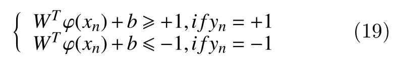
which is equivalent to

In the LS-SVM technique, optimal separation of hyper-plane can be determined to maximize the distance from every class to the hyper-plane. The optimization problem can be addressed by the following equation[28]:

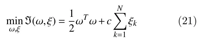
which is subjected to equality constraints,

Constructing Lagrangian is given by

with Lagrange multipliers αk≥ 0, νk≥ 0, (k=1,...,N)

After solving equation 24, the LS-SVM classifier is given by

where represents a kernel function. In this paper,radial basis kernel function has been used for the 2-class problem. The kernel function is defined by

Random forest (RF) classifier

RF are a combination of tree predictors and emerged as an efficient tool in classification for the reason that they do not overfit. The accuracy of the RF classifiers improves with injection of right type of randomness, the individual predictor's strength and their correlations. RFs produce results competitive with boosting and adaptive bagging without change in the training set. With the knowledge of the construction of single classification trees, RF develops several trees for classification. To classify a new sample, the values of the sample are assigned to the trees in the forest. Then, every tree gives a classification, which means it actually "votes" for that class. The forest chooses the classification having the most votes as compared to all the trees in the forest[29].

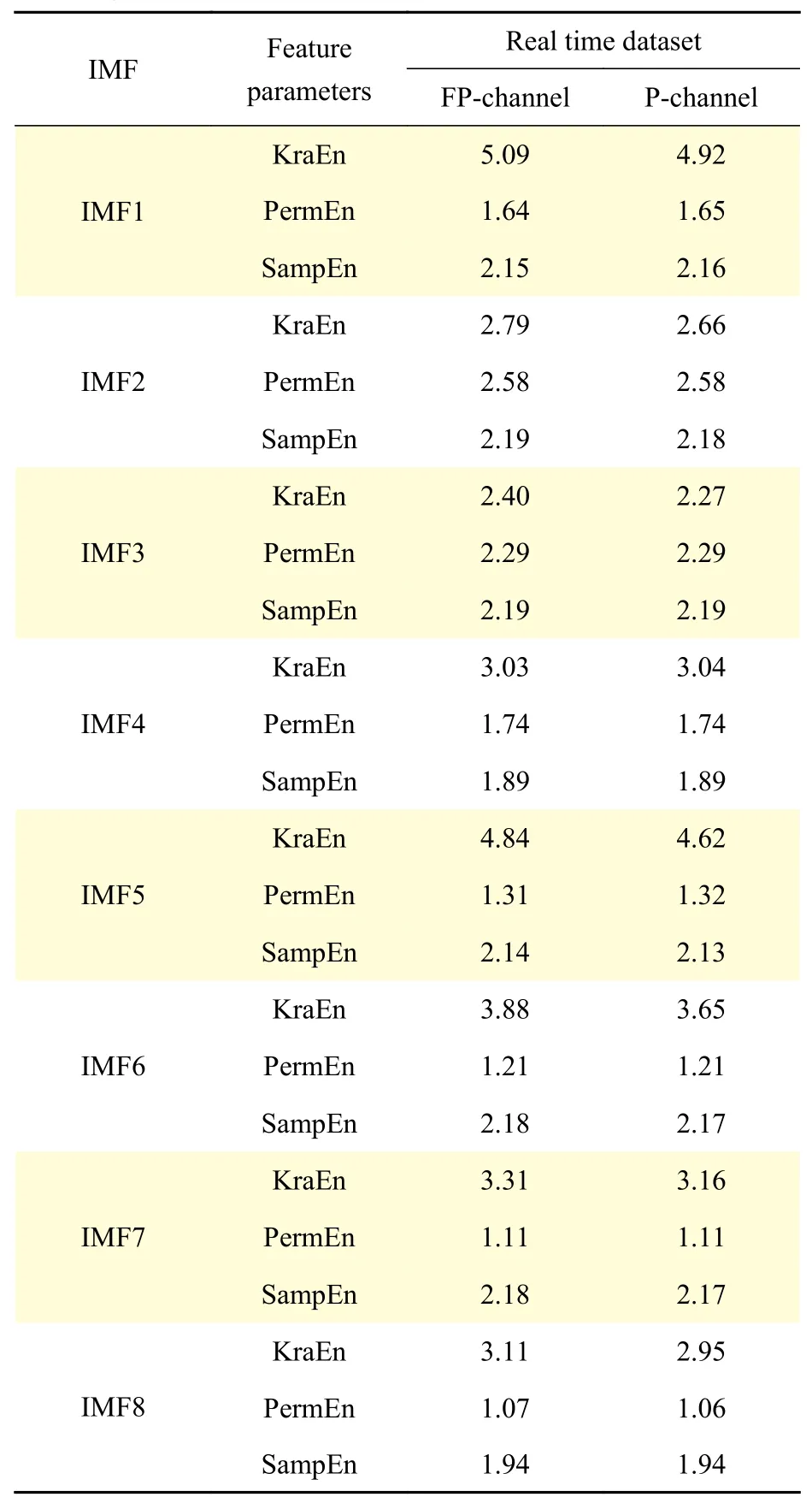
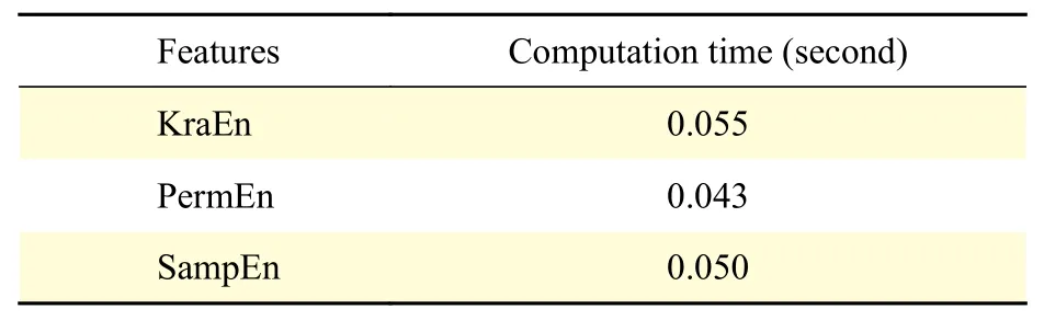
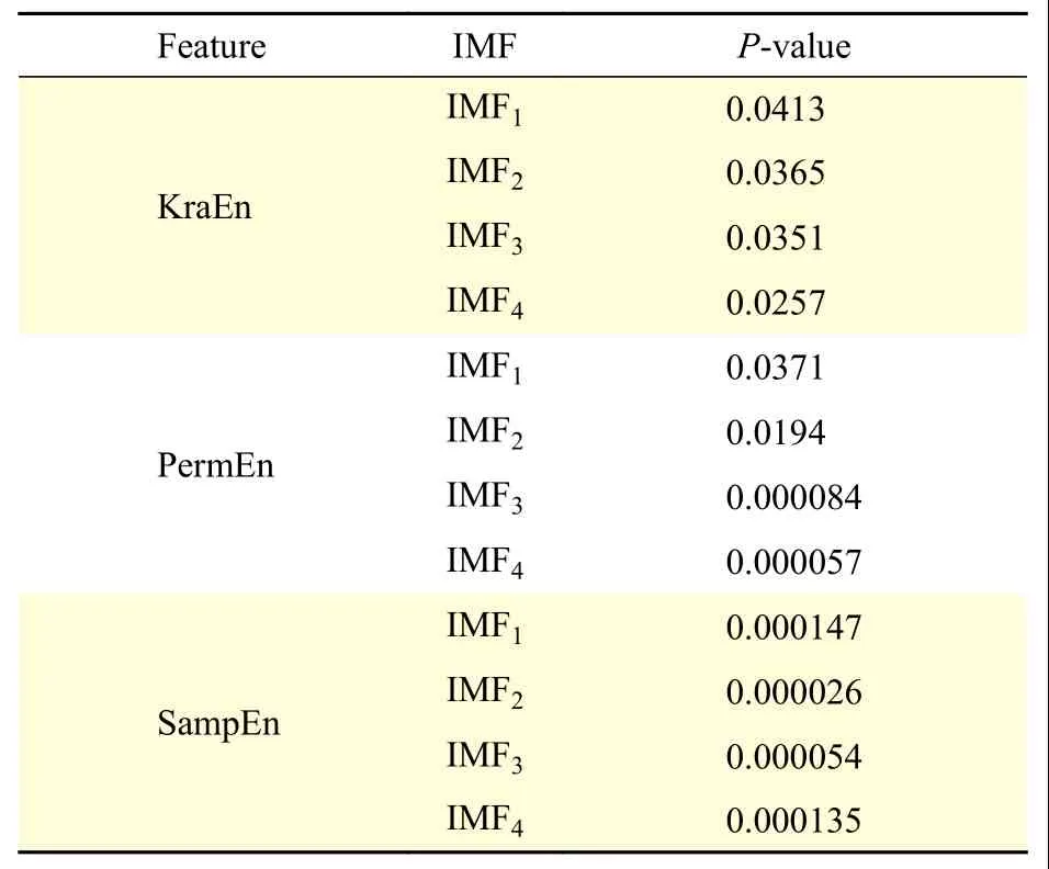
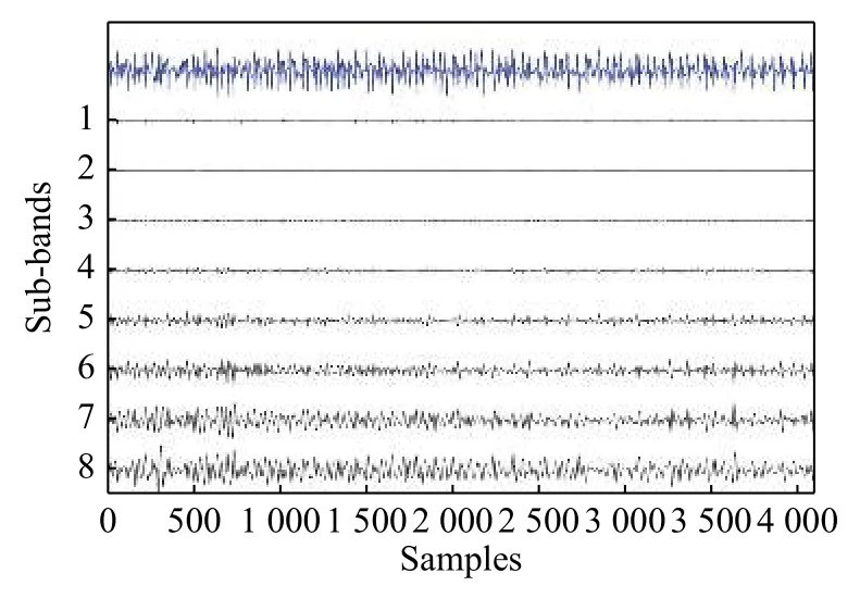
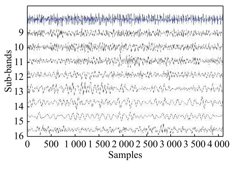
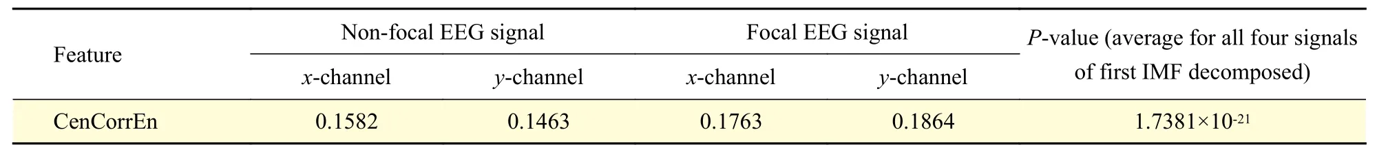
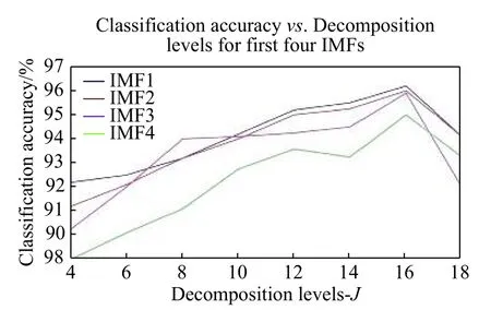
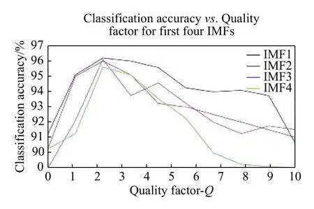
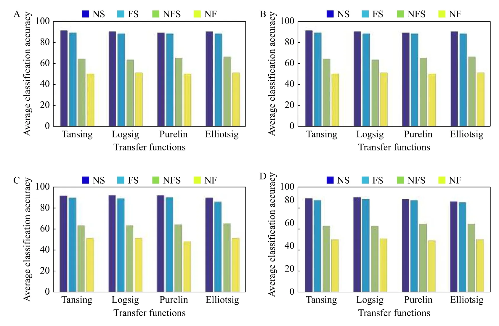
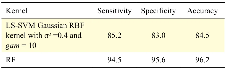
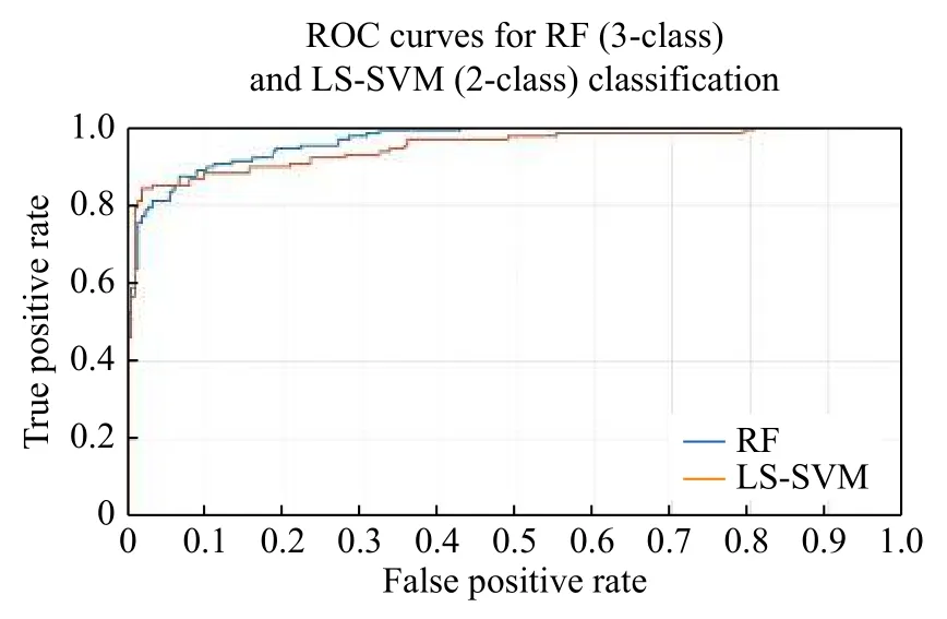
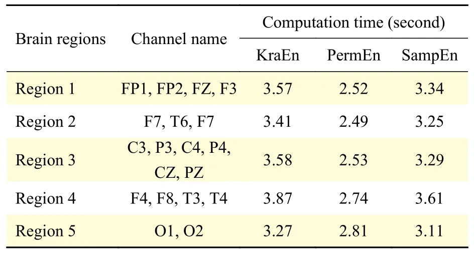
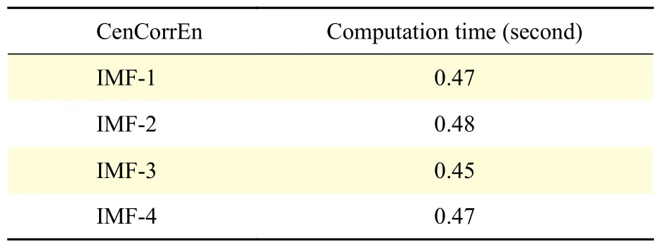
ForMinput variables, a numberm<

In this work, 3-class problem (normal, pre-ictal, and ictal) is designed using RF classifier due to its suitability in multiclass classification over SVM. A random vector?nis used to assign thenthtree. The number of features in the training set arexN=100. The tree classifierC(xN,?n) for 3-class problem was developed using feature samples and the random vector.

Results

The experiment used datasets with difference in signal from adjacent channels. Differencing stabilized the mean of EEG signals by eliminating changes in the level of the signals, and so eliminated seasonality and drift. Firstly, signals from various channels were decomposed into band-limited, oscillatory and symmetric IMFs. In this work, signal pairs of seizure and non-seizure EEG signals were decomposed using EEMD algorithm to obtain 8 IMFs. A value of 0.4 for standard deviation error and 10 for ensemble number were selected for EEMD decomposition. Three entropy parameters namely, KraEn, PermEn, SampEn were computed for the 8 IMFs. Since maximum oscillatory information about the underlying signal is obtained from the first few IMFs[18], selection of the first four IMFs were made for TQWT decomposition.Accuracy, Sensitivity, Specificity and Receiver Operating Characteristics (ROC) are standard evaluation parameters for machine learning algorithms and have been used to analyze the performance of a classifier. The resulting observations of 3 different maximum entropy feature values derived from 8 IMFs of real time dataset are shown inTable 1.

A total of 2 562 samples of normal and seizure EEG dataset were considered due to computational complexity[30]. However, by employing EEMD, the feature set for 2 562 samples of the normal and seizure EEG signals had been considered and found computationally efficient with an average computation time of 11.63 seconds. The algorithm was tested using MATLAB 9.0.1 tool on Intel ?CoreTMi5-7200 U CPU @ 2.5 GHz with 8 GB RAM. The computation time was obtained for the entire 2 562 samples for each of the entropy features and is depicted inTable 2.The table shows the average values of computation time for randomly chosen 100 data samples from both signal classes. The minimum average time for computation of KraEn, PermEn, and SampEn was 0.042 for each IMF. The computation time depicts the potential of the proposed EEG classification algorithm in real time hardware implementation. The CenCorrEn of the 16thsub-band of TQWT is separately computed and computation time of the same has not been considered in this paper.

The KraEn estimated the Shannon entropy of the dataset using k-nearest neighboring sample. The KraEn of IMFs with Euclidean distance produced a valuable feature set for 2-nearest neighbor sample.The PermEn computes the permutation entropyHof the IMFs using permutation ordern, time lags fromtauand a method to treat equal values. These parameters describe the accuracy of the values in the IMF data series by the number of decimal places. In this work, the value ofn=1, 2, 3 were considered to experiment and the optimum PermEn feature set was obtained forn=3, for which maximum classification accuracy has been achieved. The SampEn computes sample entropy of input signal vector for maximum template lengthM. The default value ofM=5.Experimental values ofM=1, 2, 3, 4, 5 have been employed in this work. When the SampEn is estimated forM=1, ...,M-1, the feature set size increases with standard error estimates (se), and therefore the number of matches form= 1, ...,Mandm=0, ...,M-1 are computed separately. In this work the maximum accuracy of RF classifier has been reported for SampEn feature vector computed forM=1.

Initially, 100 EEG signals (50 each from normaland seizure) were selected to compute entropy features. Using 8 IMFs and 3 entropy parameters the size of the feature vector became 42×1 000. In the next step, to minimize the classifier complexity,selection of the IMFs containing the best possible entropy for further decomposition using TQWT was achieved using Student'st-test (P≤0.05)[31]. The reduced feature set after performing the test was of 12×1 000 size is shown inTable 3.

Table 1 The maximum value of the entropy features computed for fourteen IMFs of real time datasets sample EEG signals

Table 2 Computation time for entropies of IMFs

Further, the pair of IMFs was decomposed using TQWT for various values ofQandJ. The maximum classification accuracy was obtained for subband16of IMF pairs IMF1, IMF3, and IMF4forQ=3 andJ=16.The minimum value ofrwas selected as 3. The decomposition of the 1stIMF from seizure difference signal into the 1stto 8thand 9thto 16thsub-bands are shown inFig. 6and7, respectively.

For CenCorrEn features computed from the 16thsub-band are shown inTable 4.

The computation of CenCorrEn was done using Laplacian kernel in ITL toolbox available online(http://www.sohanseth.com/Home/codes). The MATLAB function computes the parametric CenCorrEn between two IMF vectors,IMFxandIMFy, where 'x'and 'y' are positive integers. In this work, the maximum entropy was obtained for IMF34for default parameter of [1, 0]and kernel size (kSize) =1. The CenCorrEn was computed for these IMF pairs to form the final feature set which is of size 16 × 1 000. To select optimum values ofQandJusing CenCorrEn,experiments were performed to evaluate classification accuracy for various values ofQandJof TQWT. The LS-SVM classifier was implemented in MATLAB using LS-SVM toolbox available online(http://www.esat.kuleuven.be/sista/lssvmlab/).

The selection of optimum value ofQandJwas experimented by taking only CenCorrEn features that produced the highest classification accuracy. Further,the values ofJare varied by keepingQ=3. The maximum possible value ofJwithQ=3 is 16. Hence,the value ofJwas tested from 4 to 18 and CenCorrEn was computed for each sub-band. Then, the classification was performed by varying value ofJfrom 4 to 18. The plot of classification accuracy versus values ofJis shown inFig. 8.

It was observed that atJ=16, maximum classification accuracy is obtained. The fixed value ofJ=16 was then used to test the value ofQfor maximum accuracy. The variation of accuracies withQis shown inFig. 9.

Table 3 Feature set selected after performing Student's ttest of the raw feature space

Fig. 6 The 1st to 8th sub-bands of seizure EEG signal.

Fig. 7 The 9th to 16th sub-bands of seizure EEG signal.

Table 4 CenCorrEn features derived from the 16th sub-band of first IMF of 'x' and 'y' channel signal of non-focal and focal EEG

The use of various transfer functions in MLPNN,namely, "tansig", "logsig", "purelin", and "elliotsig"resulted in a comparable performance. The features were randomized before being fed into MLP network and re-trained 10 times to calculate average MSE.From the preliminary study, a number of hidden neurons were set to 10 and "tansig" was set as an input-hidden transfer function. Four training functions, namely, conjugate gradient with Powell-Beale restarts (CGB), variable learning rate backpropagation (GDX), Levenberg-Marquardt (LM),and scaled conjugate gradient (SCG) were used for the experimental study from neural network toolbox of MATLAB (MathWorks, Natick, USA).Fig. 10depicts average classification accuracy for CGB,GDX, LM, and SCG training functions for 2-class(normal-seizure) and 3-class (normal-pre-seizureseizure) problems.

It was inferred from the simulation study that the tan-sigmoid and pure linear transfer functions were optimal for input-hidden layer and hidden-output layer respectively with LM training function for network learning. Four different classification tasks were considered to assess the performance of MLPNN.

Discussion

Fig. 8 Plot of 3-class classification accuracies with J value variation for CenCorrEn feature and RF classifier.

Fig. 9 Plot of 3-class classification accuracies with Q value variation for CenCorrEn feature and RF classifier.

Fig. 10 Average classification accuracy for CGB (A), GDX (B), LM (C), and SCG (D) training functions for 2-class (NS, FS, NF)and 3-class (NFS) problem.

In the RF classifier, the increase in the number of decision trees decreases the classification errors. The number of trees was less than 50 and the errors varied with minor changes when the number of trees was larger than 250. For the RF classifier, the minimum samples for the terminal node were taken 15 and the maximum depth of tree was tuned to the crossvalidation. The maximum number of terminal nodes and maximum features to consider for split was selected based on the value of square root of the total features. However, values up to 30%–40% of the total number of features were tested to check over-fitting.The 10-fold cross validation and split of dataset into 70% train and 30% test group for both the LS-SVM and RF classifiers resulted in classification accuracies shown inTable 5.

It was observed that the tuning of RF classifier for 3-class problem outperformed LS-SVM classifier on real time dataset. The receiver operating characteristics (ROC) curves for these two classifiers is shown inFig. 11.

The ROC curves depict that the proposed method improved the RF classifier performance significantly from 84% to 96% for multichannel data samples. The computation time for the entropy calculation of all four entropy parameters is shown inTable 6. Multichannel EEG analysis from all 19 channels involves a large number of samples and hence computational complex. Hence, multi-channel signals are grouped in 5 regions and the average of signals from these regions is considered without reducing the number of channels.Table 6shows computation time of 3 entropy parameters for average of signals from brain regions.

It was observed that average computation time of 3.54, 2.62 and 3.32 seconds is required for SampEn,PermEn and KraEn. As shown inTable 7, the computation time for CenCorrEn is relatively small(0.47 seconds) as it is computed only for the 1stand 16thsub-band of TQWT decomposed IMFs.

InTable 8, the results of recent algorithms in EEG research are compared with the proposed method. In the comparison experiment, it was found that the proposed joint algorithm shows approximately 2% of improvement in classification accuracy. Besides, a comparative experiment using a basic feature extraction method using discrete wavelet transform(DWT) based entropy features fed to RF classifier results in 87% classification accuracy, while the proposed joint EEMD-TQWT results an improvement of 9.2% accuracy. This study was carried to verify the effectiveness of the proposed model with baseline method.

Finally, the joint EEMD-TQWT and RF algorithms for feature extraction and classification respectively have been implemented using an embedded system.

The EEG signal is captured with a low cost 5-channel EMOTIV INSIGHT EEG sensor. The sensor kit records EEG from 5 channels, namely, AF3, AF4,T7, T8, Pz with 2 references in the common mode sense (CMS) active electrode/driven right leg (DRL)passive electrode noise cancellation configuration.With a data transmission rate of 128 samples/sec/channel, the recorded signal is available for decomposition and entropy feature extraction with the Raspberry pi (RPi) module. The signals from each channel are processed by algorithms implemented using inbuilt Python language for a RPi model-B V1.2. The system works as an independent seizure detection module by employing the proposed algorithms. The stand alone system may help patients/neurologists in providing them with first-hand information about the diagnosis of the seizure disorders. The limited number of channels used in diagnosis of seizures is a major challenge in this system. The use of 5-channel EEG device performs better for generalized epileptic seizure. This limitation can be corrected in future by employing wired 32-channel EEG recording instrument to acquire EEG signals from the entire scalp.

Table 5 Classification performance of LS-SVM and RF classifiers (%)

Fig. 11 Receiver operating characteristic curves for RF (3-class) and LS-SVM (2-class) classifier obtained using CenCorrEn features.

Table 6 Computation time for 3 entropy parameters of 4 000 samples (23 seconds) EEG signals from 19 channels

Table 7 CenCorrEn is separately computed only for the first 4 IMFs, each IMF's 1st and 16th sub-band after TQWT decomposition)

Table 8 Comparison of classification performance

Epilepsy is a chronic brain disorder with recurrent seizures and associated disorders. The AEDs and surgical procedures are conventional ways to control seizures in case of drug resistant epilepsy. In such cases, the non-invasive seizure detection plays a vital role in automated diagnosis of epilepsy and needs systematic study and development of signal processing algorithms. In this work, a technique to categorize seizure and normal EEG signals using the tuning ofQ-factor in the wavelet transform is explored. Initially, EEMD is used to decompose raw EEG signals into band-limited IMFs. Based on highest values of three entropy parameters namely, KraEn,PermEn, and SampEn, IMFs are selected for further decomposition using TQWT. The CenCorrEn is then computed for the 1stand 16thsub bands of selected IMFs. This ensures a more relevant feature space in classifying bivariate signals. The values of TQWT parametersQ=3,r=3, andJ=16 have produced optimum classification performance. The joint EEMD-TQWT method has generated highest classification accuracy of 96.2% for RF classifier when compared to MLPNN and LSSVM. A compact low cost embedded system developed using optimum feature extraction and classification algorithms may find application in automated seizure diagnosis.

Acknowledgments

The authors are grateful to Dr. M. D. Mohire, MD,DM (Neurology), Neuro-physician, Mohire's Neurology Center & Research, Kolhapur,Maharashtra, INDIA for observing the results and providing the EEG dataset for experimentation. We also thank the developers of open source ITL toolbox and TQWT toolbox in MATLAB.