Christian Vérard, Cyril Hochard, Peter O. Baumgartner, Gérard M. Stampfli

Université de Lausanne (UNIL), Institut des Sciences de la Terre (ISTE), Geopolis, Ch-1015 Lausanne, Switzerland

Abstract A full global geodynamical model over 600 million years (Ma) has been developed at the University of Lausanne during the past 20 years. We show herein how the 2D maps were converted into 3D (i.e., full hypsometry and bathymetry), using a heuristic-based approach. Although the synthetic topography may be viewed as relatively crude, it has the advantage of being applicable anywhere on the globe and at any geological time. The model allows estimating the sea-level changes throughout the Phanerozoic, with the possibility, for the first time, to flood accordingly continental areas. One of the most striking results is the good correlation with “measured” sea-level changes, implying that long-term variations are predominantly tectonically-driven. Volumes of mountain relief are also estimated through time and compared with strontium isotopic ratio (Sr-ratio), commonly thought to reflect mountain belt erosion. The tectonic impact upon the general Sr-ratio trend is shown herein for the first time, although such influence was long been inferred.

Key words palaeogeography, reconstruction, hypsometry, bathymetry, sea-level, Sr-ratio, tectonic-climate relationship

1 Introduction*

Long-term global climatic indicator variations such as sea-level or87Sr/86Sr (Sr-ratio) isotopic changes are poorly understood because of a number of potential driving mechanisms involved. In particular, it is difficult to distinguish between the impacts of tectonically-driven versus climatically-driven factors.

Estimated sea-level variations throughout the Phanerozoic are matter of debate. Although there is consensus concerning on the crude shape of the curve with two maxima in the Cretaceous-Tertiary and the Ordovician-Silurian (see below), the magnitude of the fluctuation is controversial (see various models and references in Carter,1998). In the Cretaceous-Tertiary, the higher sea-levels above the present-day value are: 361 m at 84 Ma after Hallam (1984), 225±42 m at 82 Ma after EXXON Petroleum Company (1988), 266 m at 91 Ma after Haqet al.(1987)and Haq and Schutter (2008), 242 m at 86 Ma after Hallam and Cohen (1989), and 79 m at 53 Ma after Milleret al.(2005); all curves are adjusted to the same time scale following the International Stratigraphic Chart, version 2010.

Sr-ratio changes (see below) are commonly regarded as reflecting variations in mountain belt erosion, with increase in the Sr-ratio associated with exposure of old continental crust in collision zones. The processes responsible for the long-term trend of the Sr-ratio curve, however, remain unclear, although Sr variations are commonly associated with global tectonic activity (e.g., Veizeret al., 1999;McArthuret al., 2001).

Various attempts have been made to model sea-level variations on the basis of magnetic anomalies measured on the present-day oceanic sea-floor (Pitman, 1978; Kom-inz, 1984; Larson, 1991; Cognéet al., 2006; Mülleret al., 2008). However, in the absence of magnetic anomalies due to consumption of oceanic crust into subduction zones, (a) the reconstructions are subject to substantial assumptions which induce strong differences in results; (b)the resulting models extend back to 200-250 Ma, at best.

To overcome these issues, the geodynamic maps created at the University of Lausanne (now the property of NEFTEX Petroleum Consultants Ltd. with v.2011 academic reference license use to UNIL; hereafter referred to as UNIL model, v.2011; ? NEFTEX) are based on the“dynamic plate boundaries approach” (Stampfli and Borel,2002, 2004; and this study), which allows reconstructing not only continental areas but also disappeared oceanic realms (symbolized by synthetic anomalies) at a global scale. The model follows the physical principles governing plate tectonics, in which the main driving mechanisms are forces acting at plate boundaries (e.g., Forsyth and Uyeda, 1975; Zhong and Gurnis, 1995; Anderson, 2001;Conrad and Lithgow-Bertelloni, 2002; Stern, 2004; Schellartet al., 2007; and, see Doglioniet al., 2007 or Panzaet al., 2010 for an alternative point of view). Reconstructions are based on geodynamic scenarios involving tectonic processes (for instance, subduction propagation or subduction reversals), validated by analogue and numerical modelling(e.g., McKenzie, 1977; Cloetinghet al., 1982, 1984; Mueller and Phillips, 1991; Baeset al., 2011). Each reconstruction is supported by the PaleoDyn database (Hochard,2008; ? NEFTEX Petroleum Consultants Ltd., 2011) of compiled geological, palaeogeographical, and geophysical information of geodynamical interest, and confirmed by comparison with tomographic data (e.g., Hafkenscheidet al., 2006; Webb, 2012).

It is beyond the scope of the present paper to discuss each reconstruction of regional scale developed at the University of Lausanne over the past 20 years (e.g., Stampfliet al., 1991, 1998, 2001a, 2001b, 2002a, 2002b, 2003,2011, 2013; Stampfli, 1993, 2000; Stampfli and Pillevuit,1993; Stampfli and Borel, 2002, 2004; Stampfli and Kozur, 2006; von Raumeret al., 2006; Bagheri and Stampfli,2008; Ferrariet al., 2008; Moixet al., 2008; von Raumer and Stampfli, 2008; Flores-Reyes, 2009; Stampfli and Hochard, 2009; von Raumeret al., 2009; Wilhem, 2010;Vérardet al., 2012; Vérard and Stampfli, 2013a, 2013b;von Raumeret al., 2013), and how they were assembled to create the global reconstruction maps. However, 48 such global maps (i.e., the entire Earth’s surface) spanning the Phanerozoic in 5-20 Ma intervals have been created, and the techniques employed allow the quantitative determination of tectonic factors (e.g., mean oceanic ages [Ma],crustal production [km2/Ma], spreading rates [km/Ma or mm/yr],etc.; this study).

In the present paper, we show how the 2D geodynamical maps are converted into 3D topographic surfaces and how those can be used to quantify the impact of plate tectonics on sea-level and87Sr/86Sr ratio fluctuations.

2 Method — From 2D to 3D

Tectonic processes governing the present-day topography above sea-level (i.e., hypsometry/orography and bathymetry) of the Earth are complex. Whereas some tectonic-topography relationships are satisfactorily understood and are relatively straightforward to model(e.g., relationship between age and depth of oceanic seafloor), others (e.g., relief as a product of tectonics vs.erosion) are more difficult to simulate in the past. We followed a heuristic-based approach, and applied our technique to convert the 2D geodynamical maps of the UNIL model (v.2011; ? NEFTEX) into 3D topographic surfaces (or 2.5D since the conversion results in 3D surface and not a volume). Using statistical analyses,we converted the features constituting the model (e.g.,collision zones, margins, arcs, isochrones,etc.) into depth or elevation using theoretical equations that fit the presentday topographic relief. If this approach has the drawback of being relatively crude, it has the advantage of being applicable anywhere on the globe and at any geological epoch. The equations (below) are fitted on data stemming from ETOPO1 (a 1 arc-minute global relief model of Earth’s surface that integrates land topography and ocean bathymetry,i.e., 1’×1’grid map; Amante and Eakins, 2009)concerning the global topography, the sediment thickness map of Laske and Masters (1997; on-line updated version 1°×1°grid map, 2010), and will be further detailed elsewhere.

2.1 Topography of oceanic realm

When the depth values of all present-day ridges in the world are plotted against the rate at which oceanic seafloor was created, a linear relationship unveils (see Figure 1), and is:

whereZRidgeis the depth of the ridge in meter [m] as function of the accretion rate [mm/yr].

ETOPO1 relief has been re-sampled using data points from a geodetic grid, in order not to overestimate polar areas. Data from oceanic areas {Z} (in meter [m]) were cor-

rected for sediment load using an Airy model for isostasy:

However, the average density of a given sediment column {ρS} varies with the sediment thickness {hS}[m] as sediment compacts. We follow Winterbourneet al.(2009) for the calculation of {ρS}, with:

where, {φ} [unitless] is the porosity at a given depth{z} [m], {φ0= 0.56} is the porosity at z=0 m, {λ=4500 m} is the compaction decay wave length, {ρGrain=2650 kg.m-3} is the density of solid grain in sediment,{ρW= 1027 kg.m-3and ρM= 3150 kg.m-3} are the den?sity of water and asthenospheric mantle respectively. The sediment thickness is taken from the global map of Laske and Masters (1997; v.2010), but tests were also performed using the quasi?global (i.e., not full global coverage) map of the NOAA (Divins, 2003).

Bathymetric data from ETOPO1 corrected from sedi?ment load show a relationship with the age of the sea-floor basement (Figure 2). Contrary to Stein and Stein (1992),in particular, who argued for the use of two distinct plate models (a half?space cooling model (HSCM) for data younger than 20 Ma in square root of age, and a plate cool?ing model (PCM) for older data in exponential form), we consider (to be detailed elsewhere) that the PCM is more efficient in modelling depth-age dependence, with the form given by Turcotte and Schubert (2002):

where {w} is the sea-floor depth [m] as function of age{t} in million years [Ma].

Using the temperature at sea floor {T0= 0 °C}, the equation can be re?written for a given ridge depth {ZRidge}:

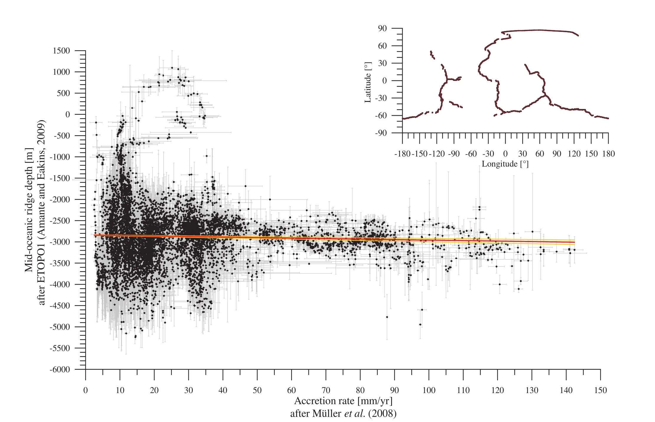
Figure 1 Mid-oceanic ridge depth [m] as function of accretion rates [mm/yr]. Red line is the linear fit and yellow curves are 95%confidence intervals (from 5000 iterations on the 7752 data points: black crosses and associated grey error bars). Inset: location of data points corresponding to mid?oceanic ridges on Earth used in the graph.

The best fit (red curve in Figure 2), using stochastic in?version method (as done for another topic by Scholeret al., 2011, for instance), is found for:

αV= 3.133 ×10-5K-1; thermal expansion coefficient.

TM= 1305.33 °C; temperature at the base of the plate.

ZLitho= 104,4 31.81 m; thickness of the cooling plate.

κ= 3.542 ×107m2.Ma-1; thermal diffusivity, withκ=（k/ （ρM× CP） ）, where k is thermal conductivity [W·m-1·K-1];ρMis mantle density [kg·m-3]; and,CPis specific heat [J·kg-1·K-1].

When worldwide bathymetric data from trenches after ETOPO1 {ZTrench} [m] are compared with predicted depth(after PCM) according to ages of the sea-floor basement entering in subduction {ZPCM} [m], a linear relationship is observed (Figure 3) and is:

Data points after ETOPO1 and the sediment map(Laske and Masters, 1997; v.2010) for abyssal plains (i.e.,12°away from any active or passive margins, and exclud?ing seamount and plateau areas) are considered to be rea?sonably fitted with a linear function of sea-floor age. As?suming the Airy model, the elevation of the sea-floor with sediment {ε.Sedt} [m] above sea-floor basement (i.e., on top of or superimposed on the PCM function given by eq.07) is:

where, {t} is the age [Ma] of the sea-floor basement.

Volcanic relief such as active hot?spots, inactive sea?mounts and plateaus are estimated as follow:

1) Oceanic relief is constructed with additional to?pography relative to sea-floor depth (after PCM), with a“plateau crest” +1537 m and the “volcanic peak” +4500 m above the given elevation, corresponding to mean value on present?day Earth (after global statistics on present?day Earth after Vérardet al., 2011 and Vérard,in preparation).

2) Continental volcanic relief is reduced (i.e., “is erod?ed”) according to the age from +1250 m for the “volcanic peak” and +1000 m for the “plateau crest” down to +293 m (median value of present?day continental hot?spot vol?canos and continental flood basalts; Vérardet al., 2011 and Vérard,in preparation). The decay function used is a PCM?like function.

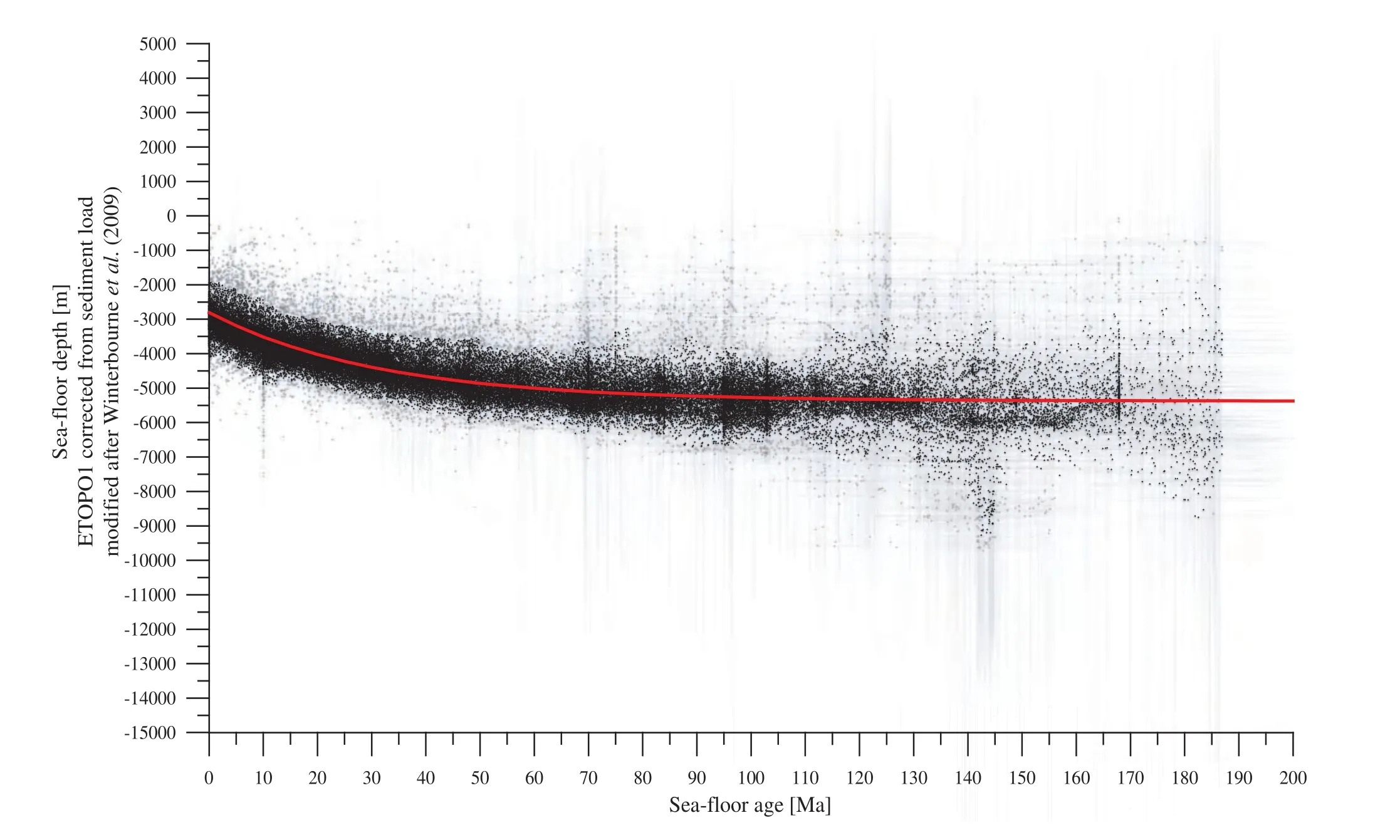
Figure 2 Bathymetric data [m] from all around the world, excluding seamount and plateau areas, corrected for sediment load versus age [Ma] of the sea-floor basement. Grey error bars are defined after the error age map of Müller et al. (2008) in x axis, and uncertain?ties on ETOPO1 data and sediment load correction in y axis. The red curve corresponds to the plate cooling model (PCM; e.g., Parsons and Sclater, 1977; Turcotte and Schubert, 2002) with the “best” fitting parameters (further discussion about this curve in Vérard et al.,2011 and Vérard, in preparation).

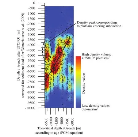
Figure 3 Worldwide bathymetric data [m] from trenches after ETOPO1 versus predicted depth (after PCM) [m] according to ages of the sea-floor at trenches. The highest densities of data follow a linear relationship (the second peak of density for theoretical depth of ca. -5500 m and depth at trench of ca. -4500 m is associated to oceanic plateau entering subduction; Vérard et al., 2011 and Vérard,in preparation for details).

2.2 Topography in transitional (ocean-continent)area

Passive margins, rifts and basins associated with aban?doned rifts are considered here to have a similar geody?namic evolution. With continental break?up, tectonic subsidence leads to rapid trough (or rift axis) deepening.Meanwhile, rift shoulders rise up. With time, however, rift shoulders thermally subside. The following cases are thus considered:

1) The rift trough subsides over a period of 7 Ma, and if the rift is abandoned, the graben is filled up with a depthage dependence following a “filling-up function” fitted on basin subsidence curve analysis (Figure 4);

2) If the rift evolves to oceanisation (in the sense of disappearance of continental crust and exposure of either denuded mantle or oceanic crust) with formation of a pas?sive margin, the continent-ocean boundary (COB) has the depth given by the PCM function;

3) Rift and passive margin shoulders are also governed by an elevation-age function, related to PCM (Figure 5).

Sediment wedges on passive margins are modelled us?ing an equilibrium profile (Figure 6) homothetically scaled in length and height according to the age of formation of the given COB.

The amount of sediment (for wedges and abysses) is modulated according to the sediment flux as defined by Fl?gelet al. (2000) (see also Hayet al., 2001; Figure 7).We note, however, that a linear relationship would also be a reasonable simplification.

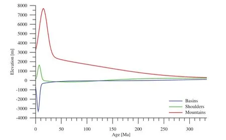
Figure 4 “Erosion” and “filling-up” functions: Blue-Depth-age dependence of basins in the case of abandoned rifts (note that if the rift turns into oceanisation, the rift axis becomes COBs, which follow the PCM equation); Green-Elevation-age dependence of rift/passive margin shoulders; Red-Elevation-age dependence of mountain crests (see text).

Figure 5 Synthetic profile for a rift or young passive margin (red curve), compared to the topography of the passive margin of Egypt in the Red Sea (black curve). Note that rift or passive margin shoulder may generate relatively high relief. Noise (blue symbols) can be added to the function (red) to test the sensibility for sea?level changes. Light blue line corresponds to the present?day sea?level.

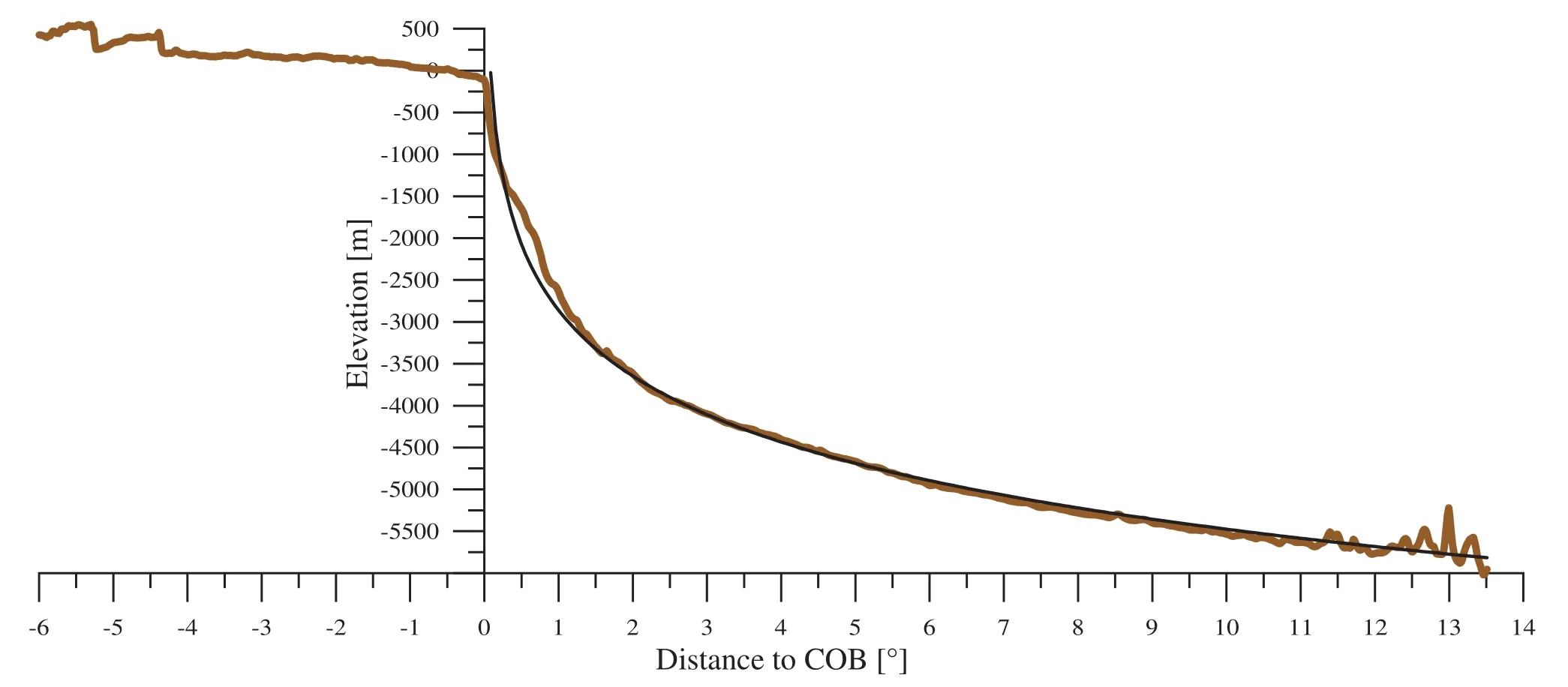
Figure 6 Profile corresponding to the sedimentary wedge of the Mauritanian passive margin (brown). The black curve is the equilib?rium profile used in the model. COB = Continent-ocean boundary.

Figure 7 Cumulative sediment flux [×1018 kg] integrated over 777 Ma after the sediment flux curve for the Phanerozoic (Inset) of Fl?gel et al. (2000) or Hay et al. (2001). Note that data are not highly departing from a linear fit (dashed red line shown as reference only), in particular for the Cenozoic-Mesozoic. The passive margin wedge equilibrium profile (Figure 6) is used as reference to homo?thetically scale in length and height of any passive margin wedges according to the age of formation of the continent-ocean boundary(COB).

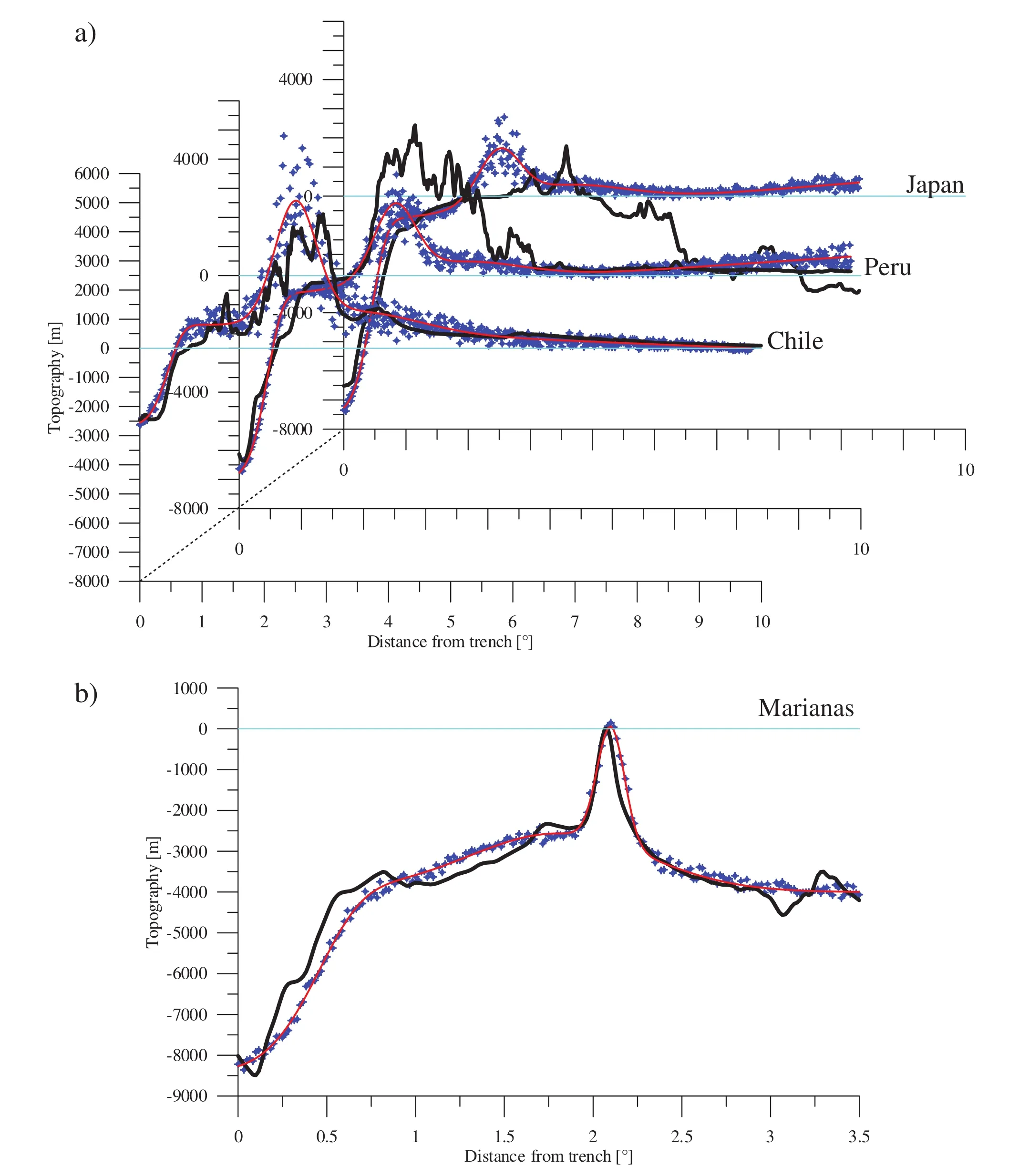
Figure 8 Synthetic profiles (red curves) for active margin (a), and intra-oceanic subduction zone (b); the black curves are the cor?responding real topography. a-Examples of profile from Chile, Peru and Japan, where the mid-oceanic ridges are subducting; b-Examples of profile from the Marianas. Note that with the same function, the depth of the trench is everywhere fairly correct. The elevation of the cordillera is correct in Chile and Japan, but not in Peru because of the difficulty to well account for the Altiplano. The position of the arc relative to the trench is fixed (2.3° away), which is reasonable in all cases here but for Japan. Noise (blue symbols)can be added to the function (red) to test the sensibility for sea?level changes and global volume of mountain belts. Light blue line corresponds to the present?day sea?level.

Active margin and intra?oceanic subduction zones are modelled with a function fitting reference cross-sections(i.e., Japan, Peru, Chile, and Mariana in Figure 8a). Trench depth (as aforementioned) and elevation of the cordillera are linked to the sea-floor age entering the subduction zone.Concerning intra?oceanic subduction zones, the height of the arc is computed to reach sub?surface (Figure 8b).

Note that abandoned arcs can be reasonably well repre?sented using a Gaussian function that fits to existing topog?raphy (e.g., Mariana abandoned arc, Lau ridge).

2.3 Topography of continental area

Mean altitude of continental plains is set constant at+240 m, which is the mean value for all present?day area on the globe comprised between 0 and 1000 m (i.e., con?sidered not to be affected by orogenies). Cratonic areas are also set with a constant value of +450 m (Figure 9). Al?though the mean continental altitude (MCA) has probably changed since continental crust appeared on Earth several billions years ago, constant values for cratons and plains over the Phanerozoic is a reasonable assumption according to Flament (2006).

Cross?sections through most orogenic belts in the world show that topography can be reasonably approximated us?ing a simple Gaussian function (example with the Alps;Figure 10). It is additionally assumed that the topographic history of an orogenic belt can be modelled using a gen?eral “erosion function” (Figure 4). Accordingly, the peak of the Gaussian function representing the mountain crests increases in height and climaxes at 15 Ma after the first signs of continent-continent collision. Then, the height of the peak decreases continuously until peneplanation.

2.4 Caveats

Due to limitations related to the structure of the UNIL plate tectonic model (v.2011; ? NEFTEX), the generated topography is only a function of the type and age of geo?logical features that comprise the model (passive margins,rifts and basins (associated with rifts), active margins, in?tra?oceanic subduction zones, abandoned arcs, active and inactive collision zones). The modelled topography is not related to date to the amount of stretching/shortening or to any local rheological aspects.

Sedimentation does not reflect local climatic variations,nor does it account for local variations in detrital input.Lakes or rivers are not taken into account on continents,and deep sea fans are not modelled here. The amount of sediment in all major deep sea fans, however, is estimated to represent less than 0.01% (order of 1014to 1015m3) of the total sediment volume in ocean.

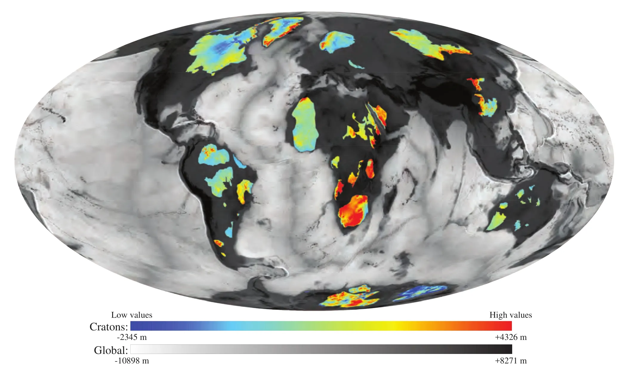
Figure 9 Location and elevation of main cratonic areas in the world (color coded). The mean value is +450 m. The global elevation is shown in black and white in background; after ETOPO1.

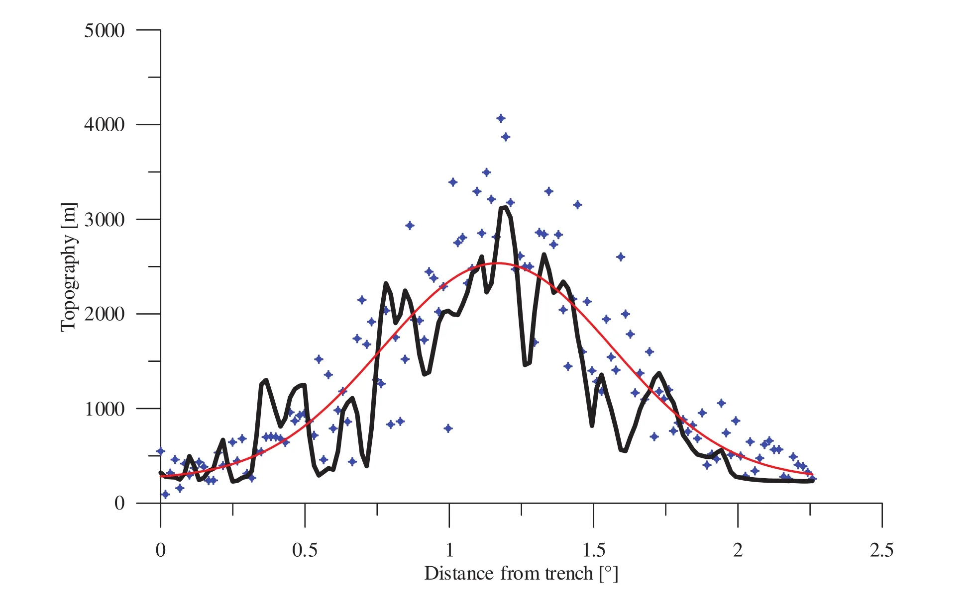
Figure 10 Synthetic profile for a collision zone (red curve), compared to the real topography through the Alps (black curve). The re?lief can be well approximated by a simple Gauss function. Noise (blue symbols) can be added to the function (red) to test the sensibility for sea?level changes and global volume of mountain belts.

The topography of arcs is not related to the velocity or angle of the subducted slab. The position of the arc is fixed relative to the trench (2.3°; present?day mean distance).

Note, finally, that effects related to post-glacial isostatic rebounds or to dynamic topography are not accounted for in the model.

2.5 Comparison with present-day data

When the synthetic topography (Figure 11c) applied to the reconstruction at 000 Ma (i.e., present?day reconstruc?tion map stemming from the evolution over 600 Ma) is compared to real topography (after ETOPO1; Figure 11a),differences (Figure 11b) are centred on zero (median value= +13.2 m; Figure 11d). Major departures from this value are related to dynamic topography, in particular in Iceland or South Africa; areas affected by post?glacial rebounds, in particular in North America and Greenland; and deep sea fans such as the Bengal fan where the sediment thickness more than 20 km is not represented.

The synthetic topography above sea?level, however,which is thought to be reliably defined since the volume of oceanic water (i.e., volume under 0 m), is 1.3343×1018m3compared to the 1.3360×1018m3obtained after ETOPO1.The amount of sediment created compares reasonably well(1.575×1017m3) with the volume (1.956×1017m3) proposed by the sediment map (Laske and Masters, 1997; v.2010).The volume of relief above +1000 m in the model is in the correct order of magnitude with 1.273×1016m3compared to the equivalent volume after ETOPO1 (2.503×1016m3).Finally, the position of the contour line at 0 m is close to the real coast?line (median value = 70.4 km; Figure 11e,and compare with Figure 11a and Figure 11c), and the ob?tained sea?level is excellent (-1 m).

The 3D development of the geodynamic reconstruction maps provides for the first time, therefore, a full synthetic topography over 600 Ma (Figure 12). The latter values show that a simple synthetic topography can be a reason?ably good approximation of the real topography, and is sufficient to test the tectonic impact on palaeo-climatic indicators.

3 Implications for sea-level and Sr-ratio variations

3.1 Comparison with sedimentation fluxes

The volume of mountain relief (in cubic?meter [m3])obtained with the 3D model can be compared (Figure 13a)with the sediment flux (in kilogram per million year [kg·Ma-1]) estimated by Fl?gelet al., (2000) for the Phanero?zoic. Because units are different, data have been standard?ised following:

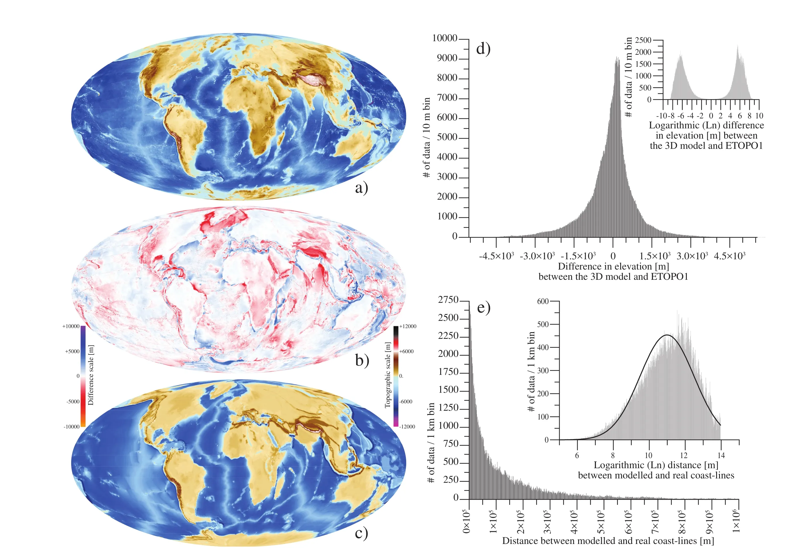
Figure 11 a-Real topography after ETOPO1 (Amante and Eakins, 2009); b-Difference in topography between the 3D model and ETOPO1 (subtraction); c-Synthetic topography resulting fromthe 3D conversion of the reconstruction map at 000 Ma (i.e., present?day); d-Difference in elevation between the 3D model and ETOPO1 (medianvalue, m= +13.2 m), the data distribu?tion is close to a Laplace function (but not strictly at the 95%confidence level; see Inset with logarithmic Xaxis); e-Distance between coast?lines location after the 3D model and ETOPO1 (m= 70.4 km; Inset with logarithmic X axis, and Gaussian “best” fit). This figure is in part derivative from the NEFTEXGeodynamic Earth Model; ? NEFTEX PetroleumConsultants Ltd., 2011.

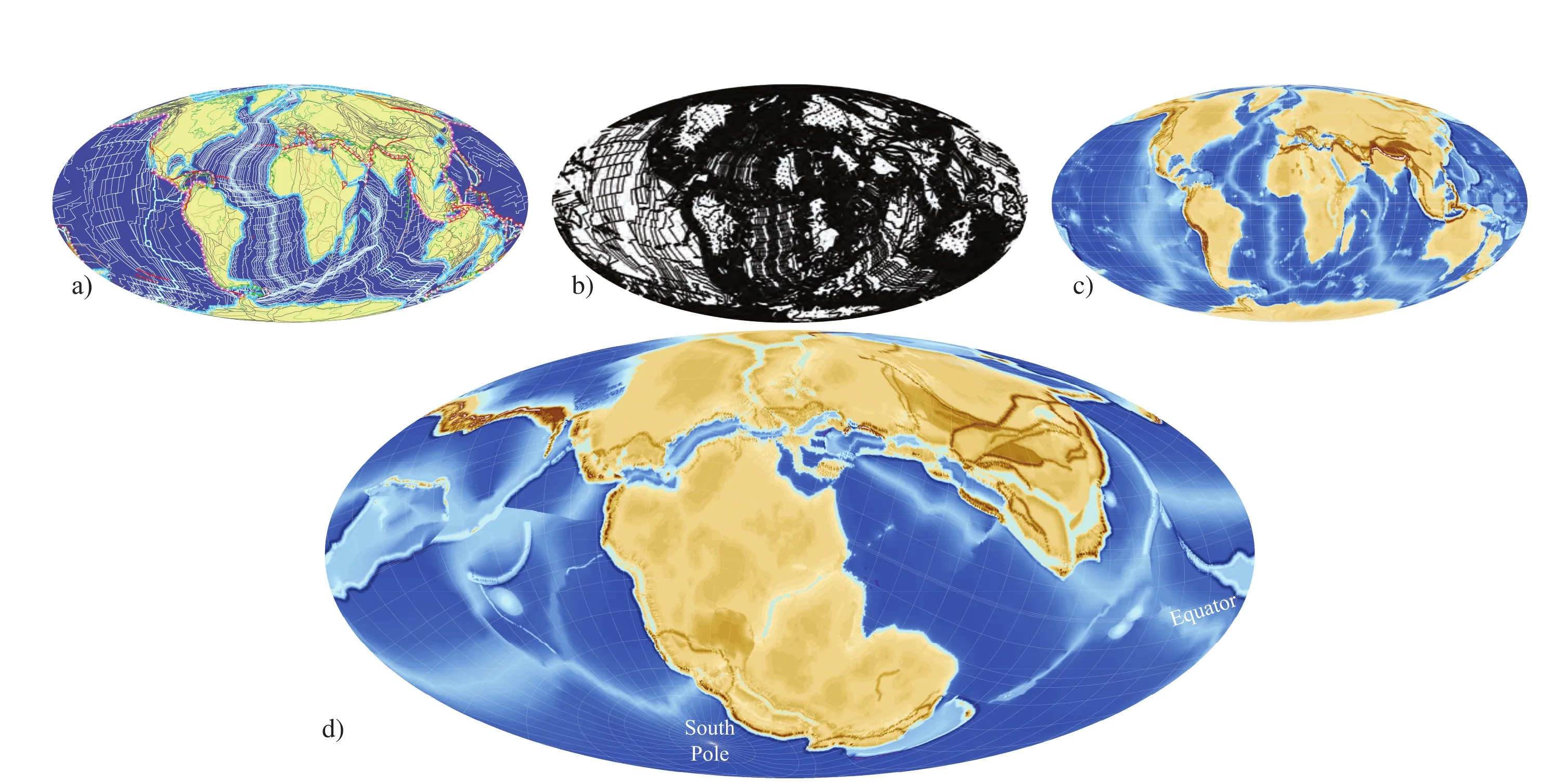
Figure 12 a-Geodynamic reconstruction map at 000 Ma (i.e., present-day configuration stemming from our 600Ma evolution); b-Data points extraction (ca. 210,000) on whichtopo?graphic function are computed; c-3D conversion model from b (i.e., from the data points extraction at 000 Ma); d-Example of 3D conversion model for the Callovian(Middle Jurassic).

whereXiis the standardised value corresponding to a given valuexi;μ is the mean value, andσ is the standard deviation of the dataset.

To first order, the two datasets correspond relatively well, except for the Late Paleozoic-Early Mesozoic. As?suming the two curves are correct, the gap between the two might be viewed as a “climatic impact” curve, with large negative values reflecting periods of intense erosion,and positive values reflecting low erosion periods. Accord?ingly, periods of intense erosion would be atca. 460 Ma,375 Ma, 150 Ma and present, whereas low erosion would be atca. 550 Ma, 400 Ma, 300 Ma, 175-225 Ma and 25 Ma (Figure 13b).

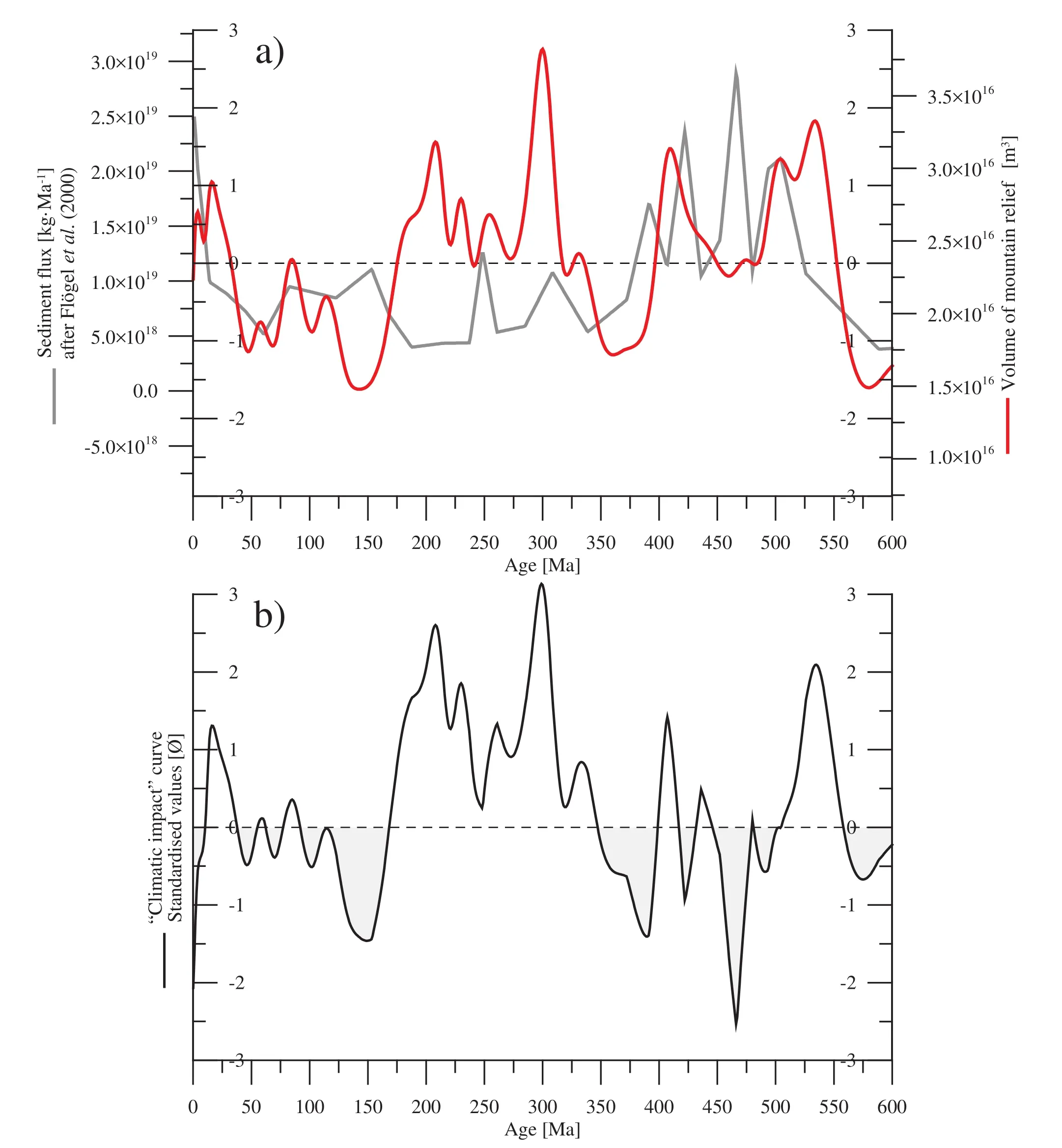
Figure 13 Comparison between the volume of mountain belts after the 3D model and the sediment flux (Fl?gel et al., 2000). Data are standardised (inner scales [-3; +3]), and Y?axes (outer scales) are adjusted correspondingly. Red-Volume of mountain relief [m3];Grey-Sediment flux [kg·Ma-1]; Black-Difference (i.e., volumes minus fluxes) between the two standardised datasets.

3.2 Comparison with Sr-ratio data

The sediment flux throughout deep time is very diffi?cult to assess, and is subject to many a priori assumptions.On the contrary, the87Sr/86Sr (Sr?ratio) data are probably the most reliable isotopic record available for the whole Phanerozoic (e.g., Fran?ois and Walker, 1992; Figure 14).In order to compare the volume of mountain belt [m3] with Sr?ratio isotopic changes [?] (i.e., unitless), data have been standardised (eq. 10; Figure 14).

Besides the apparent “cyclic” variations in the measured Sr?ratio data, the general trend of the curve is a decrease from 550 Ma toca. 150 Ma, and a more rapid increase up to present?day (Figure 14). The general trend of the curve for the volume of mountain belt is similar (see slopes of linear regression in Figure 14), although the recent increase is less pronounced. Note that strong low values prior toca.550 Ma in the curve for mountain volumes are related to a bias in the model because mountain relief older than 600 Ma are not taken into account. The relationship between continental relief and Sr?ratio trend is thus demonstrated here for the first time, although tectonic effects on Sr-ratio were long inferred in the literature.

In order to further examine the tectonic versus climatic signal in Sr?ratio record, a synthetic curve (Figures 14, 15)has been generated. The87Sr/86Sr isotopic ratio data are thought to represent values in the oceanic water reservoir,and the variations in Sr?ratio values result from input from other reservoirs (Figure 16;e.g., Fran?ois and Walker,1992; Richteret al., 1992; Berner, 1994). The present?day state of the strontium cycle can be used to model a syn?thetic Sr?ratio curve with the following parameters (com?ing from the aforementioned publications and references therein):

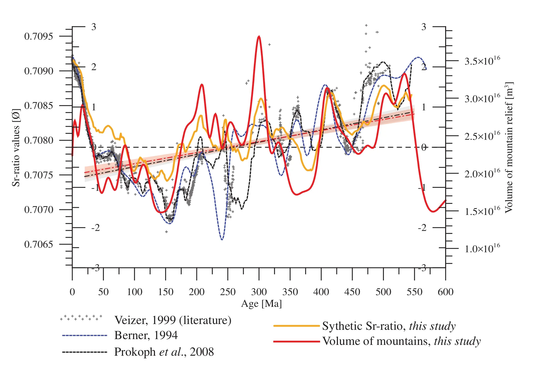
Figure 14 Various models of Sr?ratio changes for the Phanerozoic. Blue curve (Berner, 1994; and references therein). Grey data points are values from the literature (compiled by Veizer et al., 1999). Black curve (Prokoph et al., 2008). Orange, synthetic curve (case#3 in text) stemming from the model. Red, volume of mountain reliefs after 3D reconstructions. Data are standardised (inner scales [-3;+3]), and Y-axes (outer scales) are adjusted correspondingly. Dashed lines are the linear fits on the red and black curves (with colourcoded associated 95% confidence envelops). The slopes over most of the Phanerozoic [550 Ma-20 Ma] are near identical.

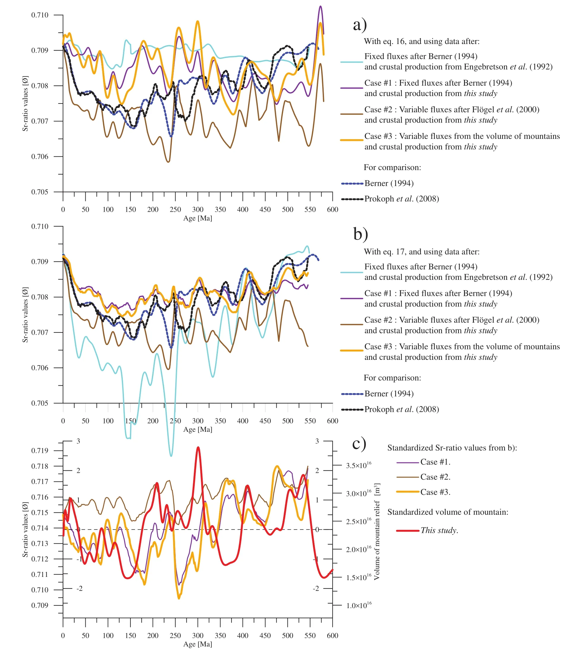
Figure 15 Synthetic Sr?ratio changes for the Phanerozoic. a-Sr?ratio curves computed after eq. 16 (see text). Light blue curve corre?sponds to the data of Berner (1994) for his GeoCarb.II model, in which he used the crustal production of Engebretson et al. (1992) and fixed fluxes, in particular fixed weathering flux {ΦW}. Purple: using fixed fluxes as Berner (1994), but with the crustal production of our 3D model (case #1). Brown: case #2, fluxes proportional to the sediment flux of Fl?gel et al. (2000) or Hay et al. (2001). Orange: case#3, fluxes proportional to the volume of mountain belts after the 3D model. Dashed curves represent measured Sr-ratio. Blue after Burke et al. (1982) and used by Berner (1994). Black after Veizer (1999) and used by Prokoph et al. (2008); b-Sr?ratio curves computed after eq. 17, i.e., by adjusting the Sr?ratio values of continental crust eroded in mountain belts; same color coding as in “a”. The minimum departure to the measured data (black curve) corresponds to data set proportional to the volume of mountain belts (case #3; orange); cf（δ） function of eq. 17, i.e., Sr?ratio values of continental crust (eroded in mountain belts) needed to obtain curves shown in “b”. The preferred solution (case #3) is shown in orange, whereas other cases are shown in purple and brown as in “a” and “b”. Data are stand?ardised (inner scales [-3; +3]), and Y?axes (outer scales) are adjusted correspondingly, to be compared with the volume of mountain belts (red curve) after the 3D model. The preferred solution (case #3; orange) is somewhat anti?correlated with the red curve (see text).

1) Typical value for unaltered mid-oceanic basalt is 0.703. Following Berner (1994), the flux of Sr due to newly created basalts is modelled as being linearly proportional to changes in crustal production {PCrust} as provided by the UNIL model (v.2011; ? NEFTEX). The flux {Ub} is:

where Fb=0.78 #1016mol/Ma, and is the present-day Sr flux from basalt;PCrust^ th and PCrust^ 0h are the crustal production [km2/Ma] stemming from the model at a given age {t} and at present {0} [Ma], respectively.

2) Sr-value for sediment is commonly of 0.708. A flux of Sr from sediment {UDia} reaches the ocean through diagenetic processes. That flux, however, is assumed to be constant with time, and is:

3) However, a flux of Sr from sediment (with a value of 0.708) is also associated with weathering. Weathering additionally affects continental crust. Typical values of Srratio for igneous rocks range fromca. 0.705 (in the range of 0.704 to 0.706; Holland, 1984) for young rocks toca.0.718 (in the range of 0.710 to 0.730; Holland, 1984) for old rocks. The present-day value is 0.715. Hence, three options have been tested (Figure 15):

(1) Following Berner (1994), the flux of Sr from weathering {UW} is fixed:

(2) The weathering flux {UW} is chosen proportional to the sediment flux curve proposed by Fl?gelet al. (2000):

where USed^th and USed^0h are the detrital sediment flux (in kg/Ma) at a given age {t} and at present {0}, respectively.

(3) The weathering flux {UW} is set proportional to the volume of mountain belts provided by our model:

where VCol^th and VCol^0h are the volume of mountain belts [m3] at a given age {t} and at present {0} after the 3D model, respectively.

In all cases,F =1.7#1016mol/Ma and is the pre-Sed sent-day Sr flux from sediment;F =1.3#1016mol/Mount Ma, and is the present-day Sr flux from weathering of mountain belts.

The synthetic Sr-ratio value can be thus written as:

The resulting models are shown in Figure 15a. For comparison, the same computation has been performed with the data used by Berner (1994) for his GeoCarb.II model(light blue curve in Figure 15a), in which he used the crustal production of Engebretsonet al. (1992) and fixed UW.None of the curves compare well with measured Sr-ratio curves from the literature.

The discrepancy between the synthetic and the measured Sr-ratio curves likely represents variations in fluxes through time and/or variations in Sr-ratio values for each reservoir. In an attempt to present a climate-free model, we chose to keep fixed values of Sr fluxes through time, and to test the variation of Sr-ratio of the different reservoirs.Because the most substantial range of potential Sr-ratio values concerns the igneous rocks from continental crust,only this test is shown herein (Figures 14, 15b). Hence, the previous equation can be re-written:

where f^dh is 0.718 for the maximum departure between the two curves, andf^dh is 0.715 for a null departure as for present-day.

With the above correction, the coefficients of correlation between the measured data (Prokophet al., 2008) and Sr-models are 75.2% with fixed {UW} (case #1), 38.6%with {UW} related to the sediment flux (case #2), and 82.2% with {UW} related to the volume of mountain belts (case #3). The Sr-ratio values needed for the above correction in case #3, in particular, makes sense when compared with the volume of mountain relief (Figure 15c). The two curves are somewhat anti-correlated (the coefficient of correlation is low but clearly negative: -11.0%). This can be understood as follows: when new orogenies are forming, young granitic bodies (with low Sr-ratio values) are emplaced, whereas time is required to erode down to old(high Sr-ratio values) crustal rocks. Such hypothesis may explain the phase shift between the two curves, and suggests that the second-order variations (or apparent “cyclicity”) in Sr-ratio record is equally related to mountain erosion.

Such results, however, must be regarded with much caution, because estimated reservoirs volume, fluxes, and their temporal evolution is subject to considerable controversy, and because results are highly sensitive to the chosen values. Nevertheless, the retained solution (orange curve in Figure 14) corresponds well with measured iso-topic data.

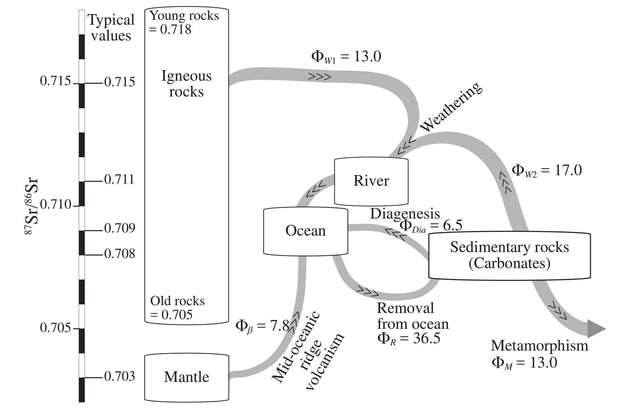
Figure 16 Schematic present-day state of strontium cycle, modified after Fran?ois and Walker (1992). The vertical axis shows the ap?proximate Sr?ratio (87Sr/86Sr) of the various reservoirs; the fluxes between reservoirs {Φ W} are given in ×109 mol/yr (or ×1015 mol/Ma).

3.3 Comparison with sea-level variations

The 3D development of the geodynamic reconstruc?tion maps has been used to determine tectonically?driven sea-level variations with, for the first time, the potential to flood continental areas in relief, throughout the Phan?erozoic.

The present?day volume of oceanic water has been placed on reconstructed topography in the past. The ob?tained sea?level variations are shown with the orange curve in Figure 17. Although the general shape of the sea?level changes is well retrieved, the amplitude is not corrected with, for instance, values of +421 m at 95 Ma.Those values, however, must be isostatically corrected be?cause the water column loads and sinks the lithosphere.When corrected for this effect (with an iterative approach to reach equilibrium), the sea?level curve (red in Figure 17) reaches +239 m above the present?day value for the Cretaceous. Although second?order variations are not vis?ible, the synthetic sea?level curve is similar to published curves, in particular with that of Haqet al. (1987) for the Cenozoic-Mesozoic as well as for the Paleozoic (Haq and Schutter, 2008). On the other hand, it departs significantly from the recently proposed sea?level curve of Milleret al. (2005) and associated error analysis (Kominzet al.,2008), potentially indicating that their results reflect local effects.

Since our model is climate?free, our results imply that long-term sea-level changes are controlled, to first order,by tectonically?driven mechanisms. Furthermore, since the volume of oceanic water is kept constant in the model and the results fit observed data, it can be inferred that no noticeable amount of water is lost in subduction processes at least since 600 Ma, and the mantle water gain and loss(e.g., Holland, 1973; Berner, 1998; Mühlenbachs, 1998;Hayet al., 2006) is in a steady state.

4 Conclusions

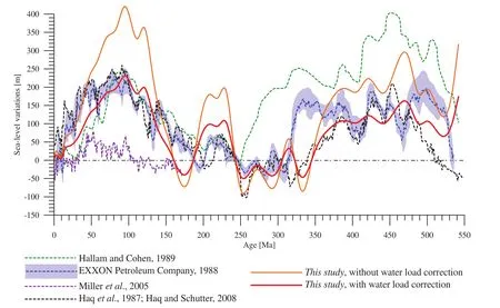
Figure 17 Various models of sea?level changes for the Phanerozoic. Blue curve after the EXXON Petroleum company (1988; unpub?lished results compiling the work of Haq et al. (1987), Posamentier and Vail (1988), and Ross and Ross (1987, 1988)); Green curve after Hallam and Cohen (1989); Black curve appending the curve of Haq et al. (1987) for the Cenozoic-Mesozoic and the curve of Haq and Schutter (2008) for the Paleozoic; Purple curve after Miller et al. (2005) spanning the Cenozoic-Mesozoic times. Sea?level curve before (orange) and after (red) isostatic adjustment due to water column loading after the 3D conversion of the geodynamic reconstruc?tion maps (this study). All curves are adjusted to the same time scale following the International Stratigraphic Chart, version 2010.

The geodynamical model developed at the University of Lausanne (UNIL) provides a palaeogeographic re?construction of the entire globe (continents and oceans)throughout the Phanerozoic. The model (now the property of NEFTEX Petroleum Consultants Ltd. with v.2011 aca?demic reference license use to UNIL) allows quantitative determination of tectonic factors on the one hand, and a full topography (above sea?level) conversion anywhere on the globe and at any geological time on the other hand.Although more sophisticated 3D modelling is needed in the future, the present version of the 3D conversion of the UNIL model (v.2011; ? NEFTEX) can retrieve the vol?ume of oceanic water, the amount of sediment in ocean,the volume of mountain relief, the location of the present?day coast?lines, and the present?day sea?level in the correct orders of magnitude.

Since the model is climate?free, it is possible to dis?tinguish between the impact of tectonically?driven versus climatically?driven factors on long?term global climatic indicators variations. The first-order decreasing trend in87Sr/86Sr (Sr?ratio) isotopic record is coherent with the decrease in volume of mountain belts (slopes in Figure 14). Although results are subject to caution, further inves?tigations using the present?day strontium cycle suggest that second?order “cyclicity” might be directly related to mountain belts, and therefore, strongly controlled by tectonics. Concerning the sea?level variations, the model shows that tectonics is the predominant factor throughout the Phanerozoic. The predicted magnitude of sea?level fluctuations agrees much better with values proposed by Haqet al.(1987) and Haq and Schutter (2008), for in?stance, than values proposed by Milleret al.(2005). The good fit between our synthetic and the proposed (Haq and Schutter, 2008) sea?level curves for the Paleozoic in par?ticular, suggest that our method (published by Stampfli and Borel, 2002; and this study) for reconstructing disap?peared oceans has merit. Such prediction is made possible because the 3D conversion allows flooding of continental area in relief during sea?level rise. Furthermore, correla?tions between tectonics and palaeoclimate indicators are probably made noticeable, because the reconstructions are made over sufficiently long period encompassing several Wilson Cycles.

Acknowledgements

We gratefully thank all members of the Prof. Stampfli’s working group for sharing their data, ideas and time with us. The Swiss National Fund (SNF) and SHELL equally acknowledged for funding the present work. We are very grateful to Prof. Zeng-Zhao Feng, Dr. Xiu-Mian Hu, Prof.Huw Davies, and Dr. Stephen Johnston for their useful and constructive comments. The geodynamical model is now the property of NEFTEX Petroleum Consultants Ltd.We gratefully acknowledge permission from NEFTEX Petroleum Consultant Ltd. to publish these derived results.