Continuous Action Reinforcement Learning for Control-Affine Systems with Unknown Dynam ics
Aleksandra Faust Peter Ruymgaart Molly Salman Rafael Fierro Lydia Tapia
I.INTRODUCTION
H UMANS increasingly rely on robots to perform tasks.A particular class of tasks that interests us are Constraint-Balancing Tasks.These taskshave one goalstate and opposing constraining preferences on the system.Balancing the speed and the quality of the task are often seen as two opposing preferential constraints.For example,the time-sensitive aerial cargo delivery task must deliver suspended load to origin as soon as possible w ith m inimal load displacement along the trajectory(Fig.1(a)).The rendezvous task(Fig.1(b))requires cargo-bearing Unmanned Aerial Vehicles(UAVs)and a ground robot to meet w ithout a predetermined meeting point.In these tasks the robotmustmanipulate and interact w ith its environment,while completing the task in a timely manner.This article considers robots asmechanical systems w ith nonlinear control-affine dynamics.Withoutknow ing their exact dynamics,we are interested in producing motions that perform a given Constraint-Balancing Task.
Control of multi-dimensional nonlinear systems,such as robots and autonomous vehiclesmust perform decision makingmany timesper second,andmustensure system safety.Yet,designing inputs to perform a task typically requires system dynam ics know ledge.Classical optimal control approaches use a combination of open-loop and closed loop controllers to generate and track trajectories[1].Another technique fi rst linearizes the system and then applies LQRmethods locally[2].A ll classicalmethods for solving nonlinear control problems require know ledge of the system dynam ics[2].On the other hand,we present a solution to an optimal nonlinear control problem when the system dynamics is unknown.
Reinforcement learning(RL)solves control of unknown or intractable dynamics by learning from experience and observations.The outcomeof RL isa control policy.Typically RL learns the value(cost)function and derives a greedy control policy w ith respect to the value.In continuous spaces,the value function is approximated[3].When actions are continuous,the greedy policymustbe approximated aswell.The downside of RL is that its sampling nature renders stability and convergence proofs challenging[3].
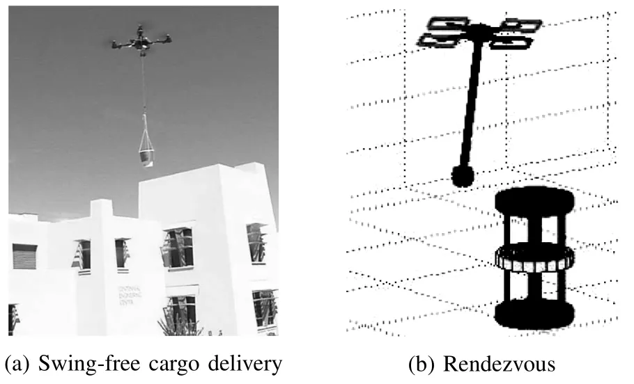
Fig.1. Evaluated tasks.
We rely on RL to learn control policy for Constraint-Balancing Tasksw ithoutknow ing the robot′sdynamics.Given the continuousstatespace,Fitted Value Iteration(FVI)approximates a value function w ith a linearmap of basis functions[4].FVI learns the linear map parametrization iteratively in an expectation-maxim ization manner[3,5].The basis function se-lection is challenging because the learning convergence is sensitive to the selection of the approximation functional space[3].Here,we select the basis functions to both fi t the task and define value function as a Lyapunov candidate function.
We extend FVI,a discrete action RL algorithm,to continuous action space to develop Continuous Action Fitted Value Iteration(CAFVI).The novelty is a jointwork w ith two value functions,state-value and action-value,to learn the control.CAFVI learns,globally to the state space,the state-value function,which is the negative of the Lyapunov.On the other hand,in the estimation step,it learns an action-value function locally around a state to estimate itsmaximum.Thismaximum is found using the new ly developed policies that divide-andconquer the problem by finding the optimal inputson each axis separately and then combine them.Not only are the policies computationally efficient,scaling linearly w ith the input′s dimensionality,but they produce consistentnear-optimal input;their outcome does not depend on the input samples used for calculation.A lthough problem decomposition via individual dimensions is a common technique for dimensionality reduction[6],this article shows that single-component policies lead to a stable system,offers three examples of such policies to turn the equilibrium into an asymptotically stable point,and characterizes systems for which the technique is applicable.The reinforcement learning agent is evaluated on a quadrotor w ith suspended load and a heterogeneous robot rendezvous task.
From the practical perspective,the article gives methods to implement an FVI w ith linear map approximation for a Constraint-Balancing Task,on control-affine systems[7]w ith unknown dynam ics and in presence of a bounded drift.These tasks require thesystem to reach agoalstate,whileminimizing opposing constraints along the trajectory.Themethod is fast and easy to implement,rendering an inexpensive tool to attempt beforemore heavy-handed approaches are attempted.
II.RELATED WORK
Efficient,near-optimalnonlinear system control isan important topic of research both in feedback controls and reinforcement learning.With known system dynam ics,[8]develops adaptive control for interconnected systems.When the system dynamics is notknown,optimal[9?11]and near-optimal[12?14]control for interconnected nonlinear systems are developed for learning the state-value function using neural networks.This article addresses the same problem,we use linearly parametrized state-value functionsw ith linear regression rather than neural networks for parameter learning.Generalized Ham ilton-Jacobi-Bellman(HJB)equation for control-affine systems can be approximately solved w ith iterative leastsquares[15].Ourmethod also learns the value function,which corresponds to the generalized HJB equation solution,through iterative minimization of the least squares error.However,we learn from samples and linear regression rather than neural networks.For linear unknown systems,[16]gives an optimal control using approximate dynam ic programm ing,while we consider nonlinear control-affine systems.Convergence proofsexist forneuralnetwork-based approximate value iteration dynamic programming for linear[17]and controlaffine systems[18],both w ith known dynam ics.Here,we are concerned w ith approximate value iteration methods in the reinforcement learning setting–w ithout know ing the system dynam ics.
In continuous action RL,the decision making step,which selects an input through a policy,becomes a multivariate optim ization.The optimization poses a challenge in the RL setting because the objective function is not known.Robots need to perform input selection many times per second;50 to 100Hz is not unusual[19].The decision-making challenges brought action selection in continuous spaces to the forefront of current RL research w ith the main idea that the gradient descentmethods find maximums for known,convex value functions[20]and in actor-critic RL[21].Our method is critic-only and because the system dynam ics is unknown,the value-function gradient is unavailable[21].Thus,we develop a gradient-free method that divides-and-conquers the problem by finding the optimal input in each direction,and then combines them.Other gradient-free approaches such as Gibbs sampling[22],Monte Carlo methods[23],and sampleaverages[24]have been tried.Online optim istic sampling planners have been researched[25?28].Specifically,Hierarchical Optimistic Optim ization applied to Trees(HOOT)[27],uses hierarchical discretization to progressively narrow the search on themost prom ising areas of the input space,thus ensuring arbitrary small error.Ourmethods find a near-optimal action through sample-based interpolation of the objective function and find the maximum in the closed-form on each axis independently.
Discrete actions FVI has solved the m inimal residual oscillations task for a quadrotor w ith a suspended load and has developed the stability conditions w ith a discrete action Markov Decision Process(MDP)[29].Empirical validation in[29]shows that the conditions hold.This article characterizes basis vector forms for control-affine systems,defines adm issible policies resulting in an asymptotically stable equilibrium,and analytically shows the system stability.The empirical comparison w ith[29]in Section IV-B shows that it is both faster and performs the task w ith higher precision.This is because the decision making quality presented here is not limited to the finite action space and is independent of the available samples.We also show w ider applicability of the methods developed here by applying them to a multi-agent rendezvous task.Our earlierwork[30]extends[29]to environmentsw ith static obstaclesspecifically foraerialcargo delivery applications,and is concerned w ith generating trajectories in discrete action spaces along kinematic paths.
III.METHODS
This section consists of four parts.First,Section III-A specifies the problem formulation for a task on a controlaffine system suitable for approximate value iteration w ith linear basis vectors.Based on the task,the system and the constraints,we develop basis functions and w rite the statevalue function in Lyapunov quadratic function form.Second,Section III-B develops sample-efficient policies that take the system to the goal and can be used for both planning and le-arning.Third,Section III-C places thepolicies into FVIsetting to present a learning algorithm for the goal-oriented tasks.Together they give practical implementation tools for solving Constraint-Balancing Tasks through reinforcement learning on control-affine systems w ith unknown dynam ics.We discuss these tools in Section III-D.
A.Problem Formulation
Consider a discrete time,control-affine system w ith no disturbances,:X×U→X,

where states areRdx,input is defined on a closed interval around origin,∈U?Rdu,du≤dx,,and:X→Rdx×Rdu,()T=1()()]is regular for,nonlinear,and Lipschitz continuous.Drift:X→Rdx,is nonlinear,and Lipschitz.Assume that the system is controllable[2].We are interested in autonomously finding control inputthat takes the system to its origin in a timely-manner while reducingalong the trajectory,whereAT=1]∈Rdg×Rdx,dg≤dxis nonsigular.
A discrete time,determ inistic fi rst-order MDPw ith continuous state and action spaces,

defines the problem.ρ:X→R is the observed state reward,and the system dynamicsis given in(1).We assume that we have access to itsgenerativemodelor samples,but thatwe do not know.In the remainder of the article,when the time stepkis not important,it is dropped from the state notation w ithout the loss of generality.
A solution to MDP is an optimal policythat maximizes discounted cumulative state reward.Thus,the objective function to maxim ize,state-value cost functionV:X→R,is

whereρkis immediate reward observed at time stepkstarting atstatex,and 0≤γ<1 a discount constant.RL solvesMDP w ithout analytical know ledge of the system dynam ics,and reward,ρ.Instead,it interacts w ith the system and iteratively constructs the value function.Using the Bellman equation[31],the state value functionVcan be recursively represented as

The state value function is an immediate state reward plus discounted value of the state the system transitions follow ing greedy policy.The action-state functionQ:X×U→R is

Action-value function,Q,is the sum of the reward obtained upon perform ing action→ufrom a statexand the value of the state that follows.Both value functions give an estimate of a value.A state-value function,V,is ameasure of state′s value,while an action-value function,Q,assigns a value to a transition from a given state using an input.Note,that RL literatureworksw ith either a state-rewardρ,or a related stateaction reward where the reward is a function of both the state and the action.We do not consider a costof action itself,thus the state-action reward is simply the reward of the state that the agent transitions upon applying action→uin the statex.Therefore,the relation between theVandQis

Both value functions devise a greedy policy:X→U,at stateas the input that transitions the system to the highest valued reachable state.

A greedy policy uses the learned value function to produce trajectories.We learn state-value function,V,because its approximation can be constructed to definea Lyapunov candidate function,and in tandem w ith the right policy it can help assess system stability.For discrete actions MDPs,(5)is a brute force search over the available samples.When the action space is continuous,(5)becomesan optim ization problem over unknown function.We consider analytical properties ofQ()for a fixed stateand knownV,but having only know ledge of the structure of the transition function.The key insight we exploit is that existence of a maximum of the action-value functionQ(),as a function of inputdependsonly on the learned parametrization of the state-value functionV.
Approximate value iteration algorithms w ith linear map approximators require basis vectors.Given the state constraint minimization,we choose quadratic basis functions

so that state-value function approximation,V,is a Lyapunov candidate function.Consequently,Vis

for a diagonal matrixΘ==diag(θ1,θ2,···,θdg),and a symmetric matrixΛ.Let us assume thatΛhas full rank.Approximate value iteration learns the parametrization Θusing a linear regression.LetΓ=?Λ.Note,that if Θis negative definite,Λis as well,whileΓis positive definite,and vice versa.Let also assume that whenΓ>0,and the system drift is bounded w ithw ith respect to Γ-norm,This characterizes system drift,conductive to the task.We empirically demonstrate its sufficiency in the robotic systemswe consider.
To summarize thesystem assumptionsused in the remainder of the article:
1)The system is controllable and the equilibrium is reachable.In particular,we use

and that()is regular outside of the origin,

2)Input is defined on a closed interval around origin,

3)The drift is bounded,

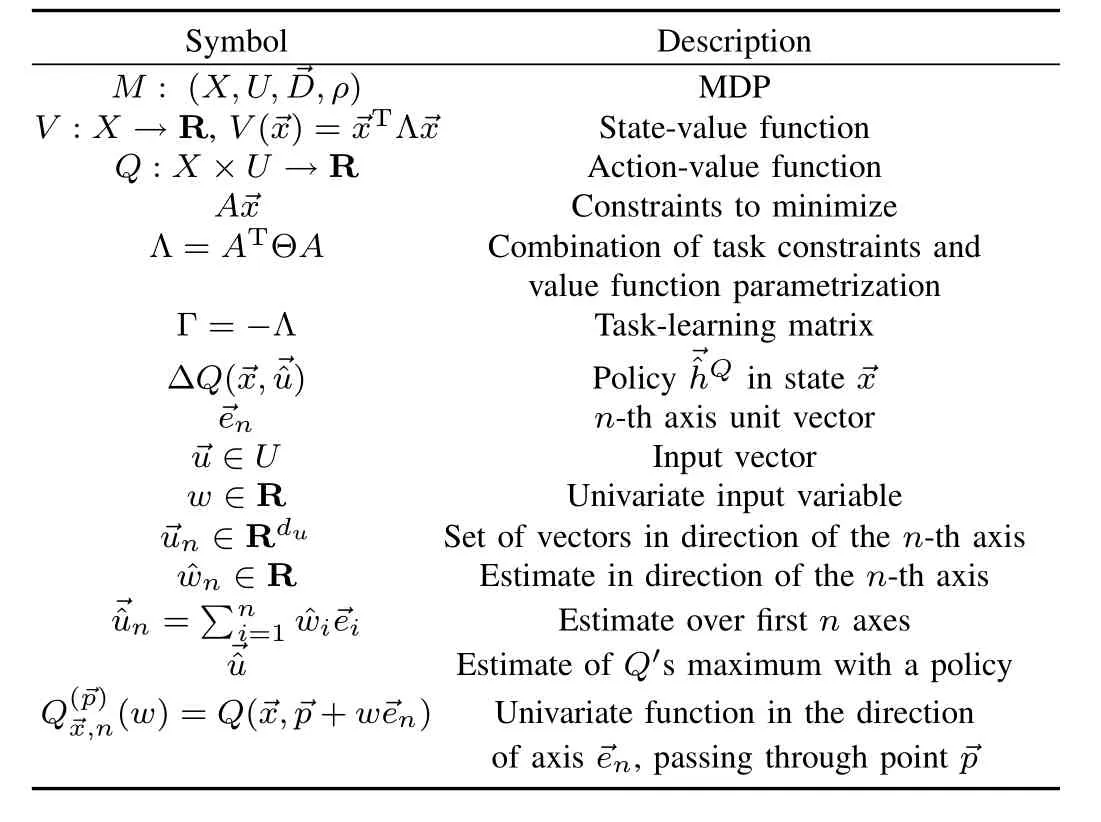
Table I presents a summary of the key symbols.TABLE I SUMMARY OF KEY SYMBOLSAND NOTATION
B.Policy Approximation
This section looks into an efficient and a consistent policy approximation for(5)that leads the system(1)to a goal state in the origin.Here,we learn the action-value functionQon the axes,and assume a known estimate of the statevalue function approximationV.For the policy to lead the system to the origin from an arbitrary state,the origin must be asymptotically stable.Negative of the state-value functionVcan be a Lyapunov function,and the value functionVneeds to be increasing in time.Thatonly holds truewhen the policy approximation makes an improvement,i.e.,the policy needs to transition the system to a state of a higher value(V(+1)>V()).To ensure the temporal increase ofV,the idea is to formulate conditions on the system dynam ics and value functionV,for whichQ,considered as a function only of the input,is concave and has a maximum.In this work,we limit the conditions to a quadratic formQ.When we establish a maximum′s existence,we approximate it by finding amaximum on the axes and combining them together.Fig.2 illustrates this idea.To reduce the dimensionality of the optimization problem,we propose a divide and conquer approach.Instead of solving onemultivariate optimization,we solveduunivariate optim izationson the axes to find a highest valued point on each axis,ui.The composition of the axes′action selections is the selection vector=[u1,···,udu]T.Thissection develops the policy approximation follow ing these steps:
1)Show thatQis a quadratic form and has a maximum(Proposition 1).
2)Define adm issible policies that ensure the equilibrium′s asymptotic stability(Theorem 1).
3)Find a sampling-basedmethod for calculating consistent,adm issible policies in O(du)time w ith no know ledge of the dynam ics(Theorem 2).
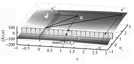
Fig.2. Example of two dimensional input and a quadratic value function.? is the optimal input, is the one selected.
Since the greedy policy(5)depends on action-valueQ,Proposition 1 gives the connection between value function(7)and corresponding action-value functionQ.
Proposition 1.Action-value functionQ(4),of MDP(2)w ith state-value functionV(7),is a quadratic function of inputfor all states∈X.When Θ is negative definite,the action-value functionQis concave and has amaximum.
Proof.EvaluatingQ()for an arbitrary state,we get

Thus,Qis a quadratic function of actionatany stateTo show thatQhas amaximum,we inspectQ′s Hessian,

The Hessian is negative definite because()is regular for all statesand Θ<0,which means thatΛ<0 as well.Therefore,the function is concave,w ith amaximum.
The state-value parametrizationΘis fixed for the entire state space.Thus,Proposition 1 guarantees that when the parametrizationΘis negative definite,the action-value functionQhas a singlemaximum.Next,we show that the right policy can ensure the progression to the goal,but we fi rst define the acceptable policies.
Definition 1.Policy approximationis adm issible,if it transitions the system to a state w ith a higher value when one exists,i.e.,when the follow ing holds for policy′s at stateΔQ()=Q()?V():
1)ΔQ()>0,for;
2)ΔQ(=0,for=
Theorem 1 shows that an adm issible policy is suffi cient for the system to reach the goal.
Theorem 1.Let=()be an adm issible policy approximation.WhenΛ<0,and the drift is bounded w ith(11),the system(1)w ith value function(7)progresses to an asymptotically stable equilibrium under policy.
Proof.ConsiderW()=?V()=TΓis a Lyapunov candidate function becauseΓ>0.
To show the asymptotic stability,aWneeds to bemonotonically decreasing in timeW(+1)≤W()w ith equality holding only when the system is in the equilibrium,=.Directly from the definition of the adm issible policy,for the state=,W(→xn+1)?W()=?Q(())+V()=V()?Q()<0.When==+1=()=because of(11)=?W(+1)=0.
Theorem 1 gives the problem formulation conditions for the system to transition to the goalstate.Now,wemove to finding sample-based adm issible policies by finding maximums ofQin the direction parallel to an axis and passing through a point.BecauseQhas quadratic form,its restriction to a line is a quadratic function of one variable.We use Lagrange interpolation to find the coefficientsofQon a line,and find the maximum in the closed form.We fi rst introduce the notation forQ′s restriction in an axial direction and its samples along the direction.
Definition 2.Axial restriction ofQpassing through point,is a univariate function

Amotivation for thisapproach is that finding amaximum in a single direction is computationally efficient and consistent.A single-component policy is calculated in constant time.In addition,the input selection on an axis calculated w ith(12)is consistent,i.e.it does not depend on the sample pointswijavailable to calculate it.This is the direct consequence of a quadratic function being uniquely determined w ith arbitrary three points.Itmeans that a policy based on(12)produces the same result regardless of the input samples used,which is important in practice where samples are often hard to obtain.
Lemma 1 shows single component policy characteristics including that a single-component policy is stable on an intervalaround zero.Later,we integrate the single-component policies together into adm issible policies.
Lemma 1.A single input policy approximation(12),for an input component,i,1≤i≤duhas the follow ing characteristics:
1)There is an input around zero that does not decrease system′s state value upon transition,i.e.,such that
3)Q,ii)?V()=0.
The proof for Lemma 1 is in Appendix A.
We give three consistent and admissible policies as examples.First,the Manhattan policy finds a point thatmaxim izesQ′s restriction on the fi rst axis,then iteratively finds maximums in the direction parallel to the subsequentaxes,passing through points thatmaximize the previous axis.The second policy approximation,Convex Sum,is a convex combination of the maximums found independently on each axis.Unlike the Manhattan policy that works serially,the Convex Sum policy parallelizeswell.Third,Axial Sum is themaximum of the Convex Sum policy approximation and nonconvex axial combinations.This policy is also parallelizable.All three policiesscale linearly w ith the dimensionsof the inputO(du).Next,we show that they are adm issible.
Theorem 2.The system(2)w ith value function(7),bounded drift(11),and a negative definiteΘ,starting at an arbitrary state→x∈X,and on a setU(10),progresses to an equilibrium in the origin under any of the follow ing policies:
1)Manhattan policy
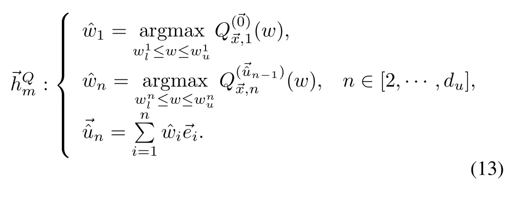
2)Convex Sum

3)Axial Sum

where

The proof for Theorem 2 is in Appendix B.
A consideration in reinforcement learning,applied to robotics and other physical systems,is balancing exploitation and exportation[32].Exploitation ensures the safety of the system,when the policy is sufficiently good and yields no learning.Exploration forces the agent to perform suboptimal steps,and the most often used?-greedy policy performs a random action w ith probability?.A lthough the random action can lead to know ledge discovery and policy improvement,it also poses a risk to the system.The policies presented here fi twell in online RL paradigm,because they allow safe exploration.Given that they arenotoptimal,they produce new know ledge,butbecause of their admissibility and consistency,their inputof choice is safe to the physicalsystem.For systems w ith independent inputs,Axial Sum policy is optimal(see Appendix C).
C.Continuous Action Fitted Value Iteration(CAFVI)
We introduced an adm issible,consistent,and efficient decision making method for learning action-value functionQlocally,at fixed state,and fixed learning iteration(whenΘ is fixed)w ithoutknow ing the system dynamics.Now,the decisionmaking policies are integrated into a FVI framework[3,5]to produce a reinforcement learning agent for continuous state and action MDPs tailored for control-affinenonlinear systems.The algorithm learns the parameterization,and worksmuch like approximatevalue iteration[5]to learn state-value functionapproximationbut the action selection uses sampling
based policy approximation on the action-value functionQ.A lgorithm 1 shows an outline of the proposed Continuous Action Fitted Value Iteration(CAFVI).It fi rst initializes
w ith a zero vector.Then,it iteratively estimatesQfunctionvalues and uses them to make a new estimate of First,we random ly select a stateand observe its reward.Line 6 collects the samples.It uniform ly samples the state space for.Because we need three data points for Lagrangian interpolation of a quadratic function,three input samples per input dimensions are selected.We also obtain,either through a simulator or an observation,the resulting statewhenis applied to.Line 7 estimates the action-value function locally,forandusing thecurrent value.Next,the recommended action is calculated,.Looking up theavailable samples or using a simulator,the system makes the transitionfromusing action.The algorithm makes a new estimate ofV().A fternsstates are processed,Line 12 finds new that m inim izes the least squares error for the new statevalue function estimatesvls.The process repeats until either converges,or amaximum number of iterations is reached.
A lgorithm 1.Continuous Action Fitted Value Iteration(CAFVI)
Input.,discount factorγ,basis function vector
Output.
2)l←1
3)while(l≤m axiterations)anddo
4)forls=1,···,nsdo
5)sample stateand observe its rewardρls
7)foralli,jdoend for{estimate actionvalue function}
8)calcu lated w ith(12)
11)end forP
13)l←l+1
14)end while
15)return
The novelties of Algorithm 1 are continuous input spaces,and the jointwork w ith both state and action-value functions(Lines 6-8),while FVIworks w ith discrete,finite input sets and w ith one of the two functions[3],but not both.A lthough the outcome of the action-value function learning(Line 8)is independent of the input samples,the state-value function learning(Line 12)depends on the state-samples collected in Line 5,just like discrete action FVI[5].
D.Discussion
Considering a Constraint-Balancing Task,we proposed quadratic feature vectors,and determined sufficient conditions forwhich admissible policiespresented in Section III-B transition the system to the goalstate obeying the task requirements.Finally,we presented a learning algorithm that learns the parametrization.There are several points that need to be discussed,convergence of the CAFVIalgorithm,usage of the quadratic basis functions,and determ ination of the conditions from Section III-A.Full conditions under which FVI w ith discrete actions converges is still an active research topic[3].It is known that it converges when the system dynam ics is a contraction[3].A detailed analysis of the error bounds for FVIalgorithmsw ith finite[33]and continuous[24]actions,finds that the FVI error bounds scale w ith the difference between the basis functional space and the inherent dynam ics of the MDP.The system′s dynam ics and reward functions determ ine the MDP′s dynam ics.We choose quadratic basis functions,because of the nature of the problem we need to solve and for stability.But,basis functionsmust fi t reasonably well into the true objective function(3)determined by the system dynam ics and the reward,otherw ise CAFVIdiverges.
The goal of this article is to present an efficient toolset for solving Constraint-Balancing Tasks on a control-affine system w ith unknown dynam ics.Using quadratic basis functions,A lgorithm 1 learns the parametrizationSuccessful learning that converges to awith all negative components,produces a controller based on Section III-B policies that is safe for a physical system and completes the task.
In Section III-A,we introduced sufficient conditions for successful learning.The conditions are sufficient but notnecessary,so the learning could succeed under laxer conditions.Done in simulation prior to a physical system control,the learning can be applied when we are uncertain if the system satisfies the criterion.When the learning fails to converge to all negative parameters,the controller isnotviable.Thus,a viable controller is possible under laxer conditions verifiable through learning;so the toolsetcan be safely and easily attempted fi rst,beforemore computationally intensivemethods are applied.It can be also used to quickly develop an initial value function,to be refined laterw ith anothermethod.
IV.RESULTS
This section evaluates the proposed methodology.We fi rst verify the policy approximations′quality and computational efficiency on a known function in Section IV-A,and then we showcase the method′s learning capabilities in two case studies:a quadrotor w ith suspended payload(Section IV-B),and amulti-agent rendezvous task(Section IV-C).
In all evaluations,the Convex Sum was calculated using equal convex coefficientsDiscrete and HOOT[27]policies are used for comparison.The discrete policy uses an equidistant grid w ith 13 values per dimension.HOOT uses three hierarchical levels,each covering one tenth of the inputsize perdimension andmaintaining the samenumberof inputs ateach level.A ll computation was performed using Matlab on a single core Intel Core i7 system w ith 8GB of RAM,running the Linux operating system.
A.Policy Approximation Evaluation
In Section III-B,we proposed three policy approximations and showed their adm issibility.To empirically verify the findings,we exam ine their behavior on known quadratic functions of two variables,ellipticalparaboloidsw ith amaximum.Table IIdepictsmaximum and minimum values forasQranges over the class of concave elliptical paraboloids.Since theΔQis always positive for all three policies,the empirical results confi rm our findings from Theorem 2 that the policies are adm issible.We also see from m inΔwthat in some cases Manhattan and Axial Sum make optimal choices,which is expected as well.Themaximum distance from the optimal input column(maxΔw)shows that the distance from the optimal input is bounded.

TABLE II SUMMARY OF POLICY APPROXIMATION PERFORMANCE.M INIMUM AND MAXIMUM OF THE VALUEGAIN(ΔQ)AND THE DISTANCE FROM THE OPTIMAL INPUT(Δw)

To further evaluate the policies′quality we measure the gain ratio between the policy′s gain and maximum gain on the action-value function(is optimal input):Non-adm issible policies have negative or zero gain ratio for some states,while the gain ratio for adm issible policies is strictly positive.The gain ratio of one signifies that policyis optimal,while a gain ratio of zero means that the selected input transitions the system to an equivalent state from the value function perspective.The elliptic paraboloids′isoclines are ellipses,and the approximation error depends on the rotational angle of the ellipse′s axes,and its eccentricity.Thus,a policy′s quality is assessed as a function of these two parameters:the rotational angleαand range of the parameterc,while parametersa,d,e,andfare fixed.Parameterbis calculated such thatb=(a?c)tan 2α.The eccentricity is depicted in Fig.3(a),w ith zero eccentricity representing a circle,and an eccentricity of one representing the ellipse degenerating into a parabola.The empty areas in the heat maps are areas where the function is either a hyperbolic paraboloid or a plane,rather than an elliptic paraboloid and has no maximum.Fig.3 displays the heatmaps of the gain ratios for the Manhattan(Fig.3(b)),Axial Sum(Fig.3(c)),and Convex Sum(Fig.3(d))policies.All policieshave strictly positive gain ratio,which gives additional empirical evidence to support the finding in Theorem 2.Manhattan and Axial Sum perform sim ilarly,w ith the best results for near-circular paraboloids,and degrading as the eccentricity increases.In contrast,the Convex Sum policy performs best for highly elongated elliptical paraboloids.
Lastly,we consider the computationalefficiency of the three policies,and compare the running time of a single decision making w ith discrete and HOOT[27]policies.Fig.4 depicts the computational time for each of the policies as a function of the input dimensionality.
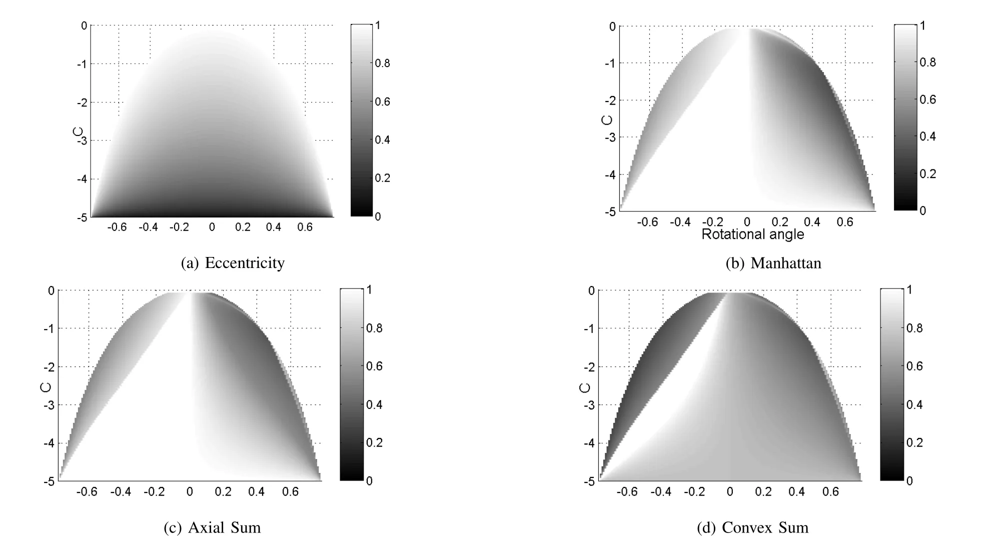
Fig.3. Eccentricity of the quadratic functions(a)related to policy approximation gain ratio(b)-(d)as a function of quadratic coefficient c,and rotation of the semi-axes.
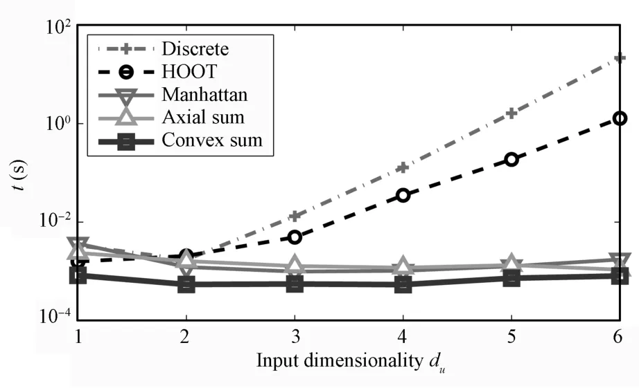
Fig.4. Policy approximation computational time per input.dimensionality.Comparison of discrete,HOOT,Manhattan,Axial Sum,and Convex Sum policies.The y-axis is logarithm ic.
Both discrete and HOOT policies′computational time grows exponentially w ith the dimensionality,while the three policies that are based on the axial maximums:Manhattan,Axial Sum,and Convex Sum are linear in the input dimensionality,although Manhattan is slightly slower.
B.Cargo Delivery Task
This section applies the proposed methods to the aerial cargo delivery task[29].This task is defined fora UAV carrying a suspended load,and seeks acceleration on the UAV′s body,that transports the joint UAV-load system to a goal state w ith minimal residual oscillations.We show that the system and itsMDP satisfy conditions for Theorem 1,and w ill assess the methods through examining the learning quality,the resulting trajectory characteristics,and implementation on the physical system.We compare it to the discrete AVI[29]and HOOT[27],and show thatmethodspresented here solve the task w ithmore precision.
To apply the motion planner to the cargo delivery task for a holonom ic UAV carrying a suspended load,we use the follow ing definition of the sw ing-free trajectory.
Definition 3.A trajectory of durationt0is said to be w ith minimal residual oscillations if for a given constant?>0 there is a time 0≤t1≤t0,such that for allt≥t1,the load displacement is bounded w ith?(ρ(t)< ?).
The MDP state space is the position of the center of the mass of the UAV=[x y z]T,its linear velocities=]T,the angular position=[ψ φ]Tof the suspended load in the polar coordinates originating at the quadrotor′s center of mass,w ith the zenith belonging to the axis perpendicular to Earth,and its angular velocities=]T.The actuator is the acceleration on the quadrotor′s body,→u=[ux uy uz]T.For the system′s generativemodel,we use a simplifiedmodel of the quadrotor-load model described in[29],which satisfies(1).is a gravitational force vector.
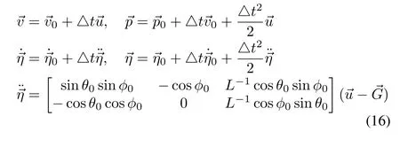
The system(16)satisfies(1).The reward function penalizes the distance from the goal state,the load displacement,and the negativezcoordinate.Lastly,the agent is rewarded when it reaches equilibrium.
The value function is approximated as a linear combination of quadratic forms of state subspacesV()=wheresatisfies the form(7),and because the learning producesθw ith all negative components,all conditions for Theorem 1 are satisfied including the drift(11).
The time-to-learn is presented in Fig.5(a).The axialmaximum policies perform an order of magnitude faster than the discrete and HOOT policies.To assess learning w ith Algorithm 1 using Manhattan,Axial Sum,and Convex Sum policies,we compare to learning using the greedy discrete policy and HOOT.Fig.5(b)shows the learning curve,over number of iterations.A fter 300 iterations all policies converge to a stable value.All converge to the same value,but discrete learning that converges to a lower value.
Finally,inspection of the learned parametrization vectors confi rms that all the components are negative,meeting all needed criteria for Theorem 1.Thismeans that theequilibrium is asymptotically stable,for adm issible policies,and we can generate trajectories of an arbitrary length.
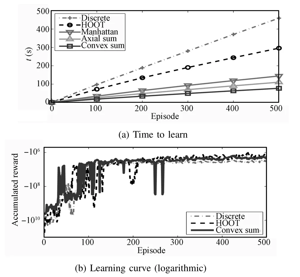
Fig.5. Learning results for Manhattan,Axial Sum,and Convex Sum,compared to discrete greedy,and HOOT policies averaged over 100 trials.Learning curves for Manhattan and Axial Sum are sim ilar to Convex Sum and are om itted from(b)for better visibility.
Next,we plan trajectories using the learned parametrizations over the 100 trials for the three proposed policies and compare them to the discrete and HOOT policies.We consider a cargo delivery task completewhen0.010m,0.025 m/s,1°,and‖≤5°/s.This is a stricter term inal set than the one previously used in[29].The input lim its are?3≤ui≤3,fori∈{1,2,3}.The discrete and HOOT policies use the same setup described in Section IV-A.The planning occurs at 50Hz.We compare the performance and trajectory characteristics of trajectories originating 3 meters from the goal state.TableIIIpresents results of the comparison.Manhattan,Axial Sum,and HOOT produce very sim ilar trajectories,while Convex Sum generates slightly longer trajectories,but w ith the best load displacement characteristics.This is because the Convex Sum takes a different approach and selects smaller inputs,resulting in smoother trajectories.The Convex Sum method plans the 9 second trajectory in 0.14 s,over 5 times faster than the discrete planning,and over 3 times faster than HOOT.Finally,30%of the discrete trajectories are never able to complete the task.This is because the term inal set is too small for the discretization.In other words,the discretized policy is not admissible.Examining the simulated trajectories in Fig.6 reveals that Convex Sum indeed selects a smaller input,resulting in a smoother trajectory(Fig.6(a))and less sw ing(Fig.5(b)).HOOT,Manhattan,and Axial Sum produce virtually identical trajectories,while the discrete trajectory has considerable jerk,absent from the other trajectories.
Lastly,we experimentally compare the learned policies.The experimentswere performed on AscTec Humm ingbird quadrocopters,carrying a 62-centimeter suspended load weighing 45 grams.The quadrotor and load position were tracked via a Vicon motion capture system at 100Hz.Experimentally,HOOT and Axial Sum resulted in sim ilar trajectories,while Manhattan′s trajectory exhibited the most deviation from the planned trajectory(Fig.7).The Convex Sum trajectory is the smoothest.Table IV quantifies themaximum load sw ing and the power required to produce the load′s motion from the experimental data.Convex Sum policy generates experimental trajectories w ith the best load sw ing performance,and w ith load motion that requires close to three times less energy to generate.
C.Rendezvous Task
The rendezvous cargo delivery task is amulti-agent variant of the time-sensitive cargo delivery task.It requires an UAV carrying a suspended load to rendezvous in sw ing-free fashion w ith a ground-bound robot to hand over the cargo.The cargo m ight be a patient airlifted to a hospital and then taken by amoving ground robot for delivery to an operating room for surgery.The rendezvous location and time are not known a priori,and the two heterogeneous agentsmust plan jointly tocoordinate their speeds and positions.The two robots have no know ledge of the dynamics and each others′constraints.The task requiresminim ization of the distance between the load′s and the ground robot′s location,the load sw ingminim ization,and m inim ization for the agents′velocities,while completing the task as fast as possible.
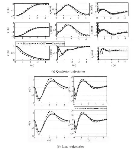
Fig.6. Comparison of simulated cargo delivery trajectories created w ith Convex Sum versus trajectories created w ith discrete greedy and HOOT policies.Trajectories for Manhattan and Axial Sum are sim ilar to Convex Sum and are om itted for better visibility.

TABLE III SUMMARY OF TRAJECTORY CHARACTERISTICSOVER 100 TRIALS.MEANS(μ)AND STANDARD DEVIATIONS(σ)OF TIME TO REACH THE GOAL,FINAL DISTANCE TO GOAL,FINAL SW ING,MAXIMUM SW ING,AND TIME TO COMPUTE THE TRAJECTORY.BEST RESULTS ARE HIGHLIGHTED.

TABLE IV SUMMARY OF EXPERIMENTAL TRAJECTORY CHARACTERISTICS.MAXIMUM SW ING AND ENERGY NEEDED TO PRODUCE LOAD OSCILLATIONS.BEST RESULTSARE HIGHLIGHTED.
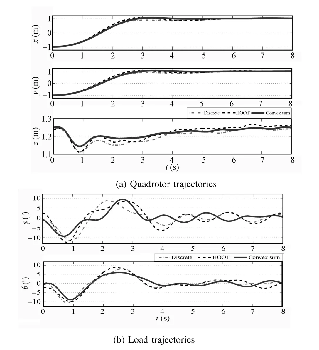
Fig.7 Comparison of experimental cargo delivery task trajectories created w ith Convex Sum versus trajectories created w ith discrete greedy and HOOT policies.Trajectories for Manhattan and Axial Sum are sim ilar to Convex Sum and are om itted for better visibility.
The quadrotor w ith the suspended load is modeled as in Section IV-B,while a rigid body constrained to two DOF in a plane models the ground-based robot.The joint state space is a 16-dimensional vector:the quadrotor′s 10-dimensional state space(Section IV-B),and the ground robot′s positionvelocity space.The input is 5-dimensional acceleration to the quadrotor′s and ground robot′s center ofmasses.The ground robot′smaximum acceleration is lower than the quadrotor′s.
Applying A lgorithm 1 w ith Convex Sum policy,the system learns the state-value function parametrizationΘthat is negative definite.Fig.8 shows both robots after two seconds.The comparison of simulated trajectories created w ith the Convex Sum and HOOT policies is depicted in Fig.9.Convex Sum finds an 8.54-second trajectory that solves the task in 0.12s.HOOT policy fails to find a suitable trajectory before reaching themaximum trajectory duration,destabilizes the system,and terminates after 101.44s.The discrete policy yields sim ilar results as HOOT.This isbecause the inputneeded to solve the task is smaller than the HOOT′s setup,and the system begins to oscillate.The rendezvous point produced w ith Convex Sum policy is between the robots′initial positions,closer to the slower robot,as expected(Fig.9(a)).The quadrotor′s load sw ing ism inimal(Fig.9(b)).The absolute accumulated reward collected while perform ing the task is smooth and steadilymaking progress,while the accumulated reward along HOOT trajectory remains significantly lower(Fig.9(c)).The rendezvous simulation shows that the proposed methods are able to solve tasks thatpreviousmethodsareunable to because the Convex Sum policy is adm issible.
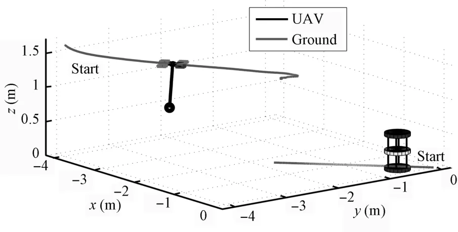
Fig.8 Cargo-bearing UAV and a ground-based robot rendezvous after 2s.
V.CONCLUSIONS
Control of high-dimensional systems w ith continuous actions is a rapidly developing topic of research.In this paper,we proposed a method for learning control of nonlinearmotion systems through combined learning of state-value and action-value functions.Negative definite quadratic state-value functions imply quadratic,concave action-value functions.That allowed us to approximate policy as a combination of its action-value function maximums on the axes,which we found through interpolation between observed samples.These policies are adm issible,consistent,and efficient.Lastly,we showed thata quadratic,negative definite state-value function,in conjunction w ith adm issible policies,are sufficient conditions for the system to progress to the goalwhileminimizing given constraints.
The verification on known functions confi rmed the policies′adm issibility.A quadrotor carrying a suspended load assessed themethod′s applicability to a physical system and a practical problem,and provided a comparison to two other methods demonstrating higher precision of the proposed method as well.The rendezvous task tested themethod in higher dimensional input spaces for amulti-agent system,and showed that it findsa solution where other twomethods do not.The results confi rm that the proposedmethod outruns currentstate-of-theart by an order of magnitude,while the experimental data revealed that the proposed method produces trajectories w ith better characteristics.
In all,we presented a solid fi rst step for an optimal control framework for unknown control-affine systems for Constraint-Balancing Tasks.Despite the applied method′s restrictive condition,the results demonstrated high accuracy and fast learning times on the practical applications.In future work,themethodology can be extended to stochastic MDPs.
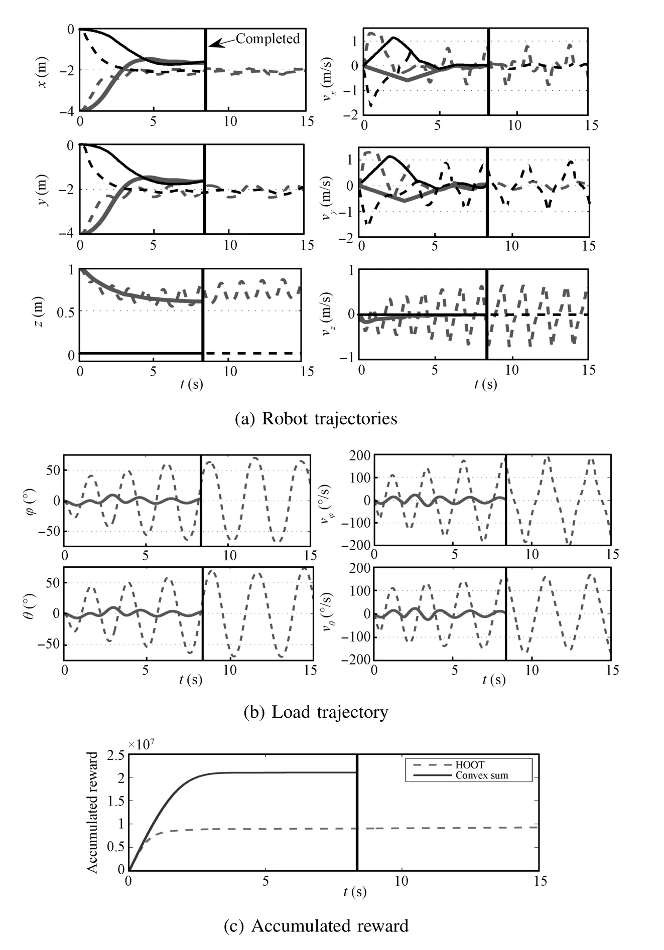
Fig.9. Comparison of simulated rendezvous task trajectories created w ith Convex Sum to trajectories created w ith discrete greedy and HOOT policies.Black solid:Convex Sum ground;Gray solid:Convex Sum aerial;Black dashed:HOOT ground;Gray dashed:HOOT aerial.
APPENDIX A PROOF FOR LEMMA 1
Proof.First,to show thatsuch thatwe pick0=0,and directly from the definition,we getAs a consequence


Third,we showQ(i)?V()=0.Since,the origin is equilibrium,the dynam ics is,i)=.Let us evaluate the dynamics atii,when=→0,

Thus,Q(ii)?V=0.
APPENDIX B PROOF FOR THEOREM 2
Proof.In all three cases,it is sufficient to show that the policy approximations are admissible.
Manhattan policy:To show that the policy approximation(13)is admissible,for=we use induction byn,1≤n≤du,w ith induction hypothesisand
First note that at iteration 1<n≤du,


Applying the induction forn=1,and using Lemma 1,


So,the induction hypothesis(A2)forn=1 holds.Assuming that(A2)holds for 1,···,n?1,and using Lemma 1,

Sim ilarly,assuming)TΛ()=→xTΛ?


Forn=du,the policy gainΔQ()=0)TΛ()=TΛand()TΛ()=0,for 1≤i≤du.But,that is contradiction w ith the controllability assumption(8),thusΔQ()>0,when=
When=,we getdirectly from Lemma 1,ΔQ()=0.This completes the proof that Manhattan policy(13)is admissible,and therefore the equilibrium is asymptotically stable.
Convex Sum(14):Follow ing the same reasoning as for the fi rst step of(A5)and(A6),we get that for all 1≤n≤du,ΔQ(nn)≥0,wherenn=and the equality holds only when

To simplify the notation,letQn=ΔQ(nn),n=1,···,du,andQ0=0.Without loss of generality,assume thatQ0≤Q1≤ ···≤Qdu.The equality only holds when(A7)holds for alln=1,···,duwhich is contradiction w ith(8).Thus,theremust be at least one 1≤n0≤du,such thatQn0?1<Qn0,and consequently 0<Qdu.
Lastly,we need to show that the combined inputcalculated w ith(14)is adm issible,i.e.,ΔQ()>0.It suffices to show thatis inside the ellipsoid0=()≥Q0}.Sim ilarly,Q1,···,Qdudefine a set of concentric ellipsoidsi=()≥Qi},i=1,···,du.Since,0?1?···?du,andi=0.Because ellipsoid0is convex,the convex combination of points inside it(14),belongs to it as well.Since,at least one ellipsoid must be a true subset of0,which completes the asymptotic stability proof.
Axial Sum policy approximation(15):is adm issible because(14)is adm issible.Formally,ΔQ(())≥ΔQ(())≥0.
APPENDIX C
OPTIMALITY CONDITIONS
Proposition 1.When()is an independent inputmatrix,A=I,and state-value function parameterizationΘisnegative definite,then Axial Sum policy(15)is optimal w ith respect to the state-value function(7).
Proof.The optimal inputis a solution toandis a solution toat statew ith respect to the state-value function(7).To show that the Axial Sum policy is optimal,?=,it is enough to show thatThis is the case when Q has the form of=,for some pxi,qxi,rxi∈R that depend on the current state→x.In Proposition 1,we showed that Q(,)=(()+()))TΘ(()+.Since there is a single nonzero element jiin row i ofmatrix.After rearranging,Q(,)=
ACKNOW LEDGEMENTS
Theauthorswould like to thank Ivana Palunko foranimation software,and Patricio Cruz for assisting w ith experiments.
[1]Levine J.Analysis and control of nonlinear systems:a flatness-based approach.Mathematical Engineering.New York:Springer,2009.
[2]Khalil H K.NonlinearSystems.New Jersey:Prentice Hall,1996.
[3]Busoniu L,Babuska R,De Schutter B,Ernst D.Reinforcement Learning and Dynamic Programm ing Using Function Approximators.Boca Raton,Florida:CRC Press,2010.
[4]Bertsekas D P,Tsitsiklis JN.Neuro-Dynam ic Programming.Belmont,MA:Athena Scientific,1996.
[5]Ernst D,Glavic M,Geurts P,Wehenkel L.Approximate value iteration in the reinforcement learning context.application to electricalpowersystem control.International Journal of Emerging Electric Power Systems,2005,3(1):10661?106637
[6]Taylor C J,Cow ley A.Parsing indoor scenes using RGB-D imagery.In:Proceeding of Robotics:Sci.Sys.(RSS),Sydney,Australia,2012.
[7]LaValle SM.Planning A lgorithms.Cambridge,U.K.:Cambridge University Press,2006.
[8]Yucelen T,Yang B-J,Calise A J.Derivative-free decentralized adaptive control of large-scale interconnected uncertain systems.In:Proceeding of the 50th Conference on Decision and Control and European Control Conference(CDC-ECC).Orlando,USA:IEEE,2011.1104?1109
[9]Mehraeen S,Jagannathan S.Decentralized optimal control of a class of interconnected nonlinear discrete-time systems by using online Ham ilton-Jacobi-Bellman formulation.IEEE Transactions on Neural Networks,2011,22(11):1757?1769
[10]Dierks T,Jagannathan S.Online optimal control of affine nonlinear discrete-time systems w ith unknown internal dynamics by using timebased policy update.IEEE Transactionson NeuralNetworksand Learning Systems,2012,23(7):1118?1129
[11]Vamvoudakis K G,Vrabie D,Lew is F L.Online adaptive algorithm for optimal control w ith integral reinforcement learning.International JournalofRobustand NonlinearControl,to be published
[12]Mehraeen S,Jagannathan S.Decentralized nearly optimal control of a class of interconnected nonlinear discrete-time systems by using online Ham ilton-Bellman-Jacobi formulation.In:Proceeding of the2010 International JointConference on NeuralNetworks(IJCNN).Barcelona:IEEE,2010.1?8
[13]Bhasin S,Sharma N,Patre P,Dixon W.Asymptotic tracking by a reinforcement learning-based adaptive critic controller.JournalofControl Theory and Applications,2011,9(3):400?409
[14]Modares H,Sistani M B N,Lew is F L.A policy iteration approach to online optimal control of continuous-time constrained-input systems.ISA Transactions,2013,52(5):611?621
[15]Chen Z,Jagannathan S.Generalized Hamilton-Jacobi-Bellman formulation-based neural network control of affine nonlinear discrete time systems.IEEE Transactions on Neural Networks,2008,19(1):90?106
[16]Jiang Y,Jiang Z P.Computational adaptive optimal control for continuous-time linear systems w ith completely unknown dynam ics.Automatica,2012,48(10):2699?2704
[17]A l-Tamimi A,Lewis F,Abu-Khalaf M.Discrete-time nonlinear HJB solution using approximate dynamic programming:convergence proof.IEEE Transactions on Systems,Man,and Cybernetics,PartB:Cybernetics,2008,38(4):943?949
[18]Cheng T,Lew is F L,Abu-Khalaf M.A neural network solution for fixed-final time optimal control of nonlinear systems.Automatica,2007,43(3):482?490
[19]Kober J,Bagnell D,Peters J.Reinforcement learning in robotics:a survey.International Journal of Robotics Research,2013,32(11):1236?1274
[20]HasseltH.Reinforcement learning in continuousstate and action spaces.Adaptation,Learning,and Optim ization.Berlin Heidelberg:Springer,2012.207?251
[21]Grondman I,Busoniu L,Lopes G A D,Babuska R.A survey of actor-critic reinforcement learning:standard and naturalpolicy gradients.IEEE Transactions on Systems,Man,and Cybernetics,Part C:Applicationsand Reviews,2012,42(6):1291?1307
[22]Kimura H.Reinforcement learning in multi-dim ensional state-action space using random rectangular coarse coding and Gibbs sampling.In:Proceeding of the 2007 IEEE International Conference on Intelligent Robots and Systems(IROS).San Diego,CA:IEEE,2007.88?95
[23]Lazaric A,RestelliM,BonariniA.Reinforcement learning in continuous action spaces through sequential Monte Carlo methods.Advances in Neural Information Processing Systems,2008,20:833?840
[24]Antos A,Munos R,Szepesv′ari C.Fitted Q-iteration in continuous action-spaceMDPs.Advances in Neural Information Processing Systems 20.Cambridge,MA:M IT Press,2007.9?16
[25]Bubeck S,Munos R,Stoltz G,Szepesvari C.X-armed bandits.The JournalofMachine Learning Research,2011,12:1655?1695
[26]Bus?oniu L,Daniels A,Munos R,Babu?ska R.Optim istic planning for continuous-action deterministic systems.In:Proceeding of the 2013 Symposium on Adaptive Dynam ic Programm ing and Reinforcement Learning.Singapore:IEEE,2013.69?76
[27]Mansley C,Weinstein A,Littman M L.Sample-based planning for continuous action Markov decision processes.In:Proceeding of the 21st International Conference on Automated Planning and Scheduling.Piscataway,NL,USA:ICML,2011.335?338
[28]Walsh T J,Goschin S,Littman M L.Integrating sample-based planning and model-based reinforcement learning.In:Proceedings of the 24th AAAI Conference on Artificial Intelligence.Atlanta,Georgia,USA:AAAIPress,2010.612?617
[29]Faust A,Palunko I,Cruz P,Fierro R,Tapia L.Learning sw ing freetrajectories for UAVsw ith a suspended load.In:Proceedingsof the2013 IEEE International Conference on Robotics and Automation(ICRA).Karlsruhe,Germany:IEEE,2013.4902?4909
[30]Faust A,Palunko I,Cruz P,Fierro R,Tapia L,Automated aerial suspended cargo delivery through reinforcement learning.In:Artificial Intelligence,2015,in press.
[31]Bellman RE.Dynamic Programming.M ineola,NY:Dover Publications,Incorporated,1957.
[32]Sutton R S,Barto A G.A Reinforcement Learning:an Introduction.Cambridge,MA:M IT Press,1998.
[33]Munos R,Szepesv′ari C.Finite-time bounds for Fitted Value Iteration.JournalofMachine Learning Research,2008,9:815?857
 IEEE/CAA Journal of Automatica Sinica2014年3期
- IEEE/CAA Journal of Automatica Sinica的其它文章
- An Improved Result of Multiple Model Iterative Learning Control
- Adaptive Iterative Learning Control for a Class of Nonlinear Time-varying Systems with Unknown Delays and Input Dead-zone
- Robust Adaptive Model Tracking for Distributed Parameter Control of Linear Infinite-dimensional Systems in Hilbert Space
- Event-Triggered Optimal Adaptive Control Algorithm for Continuous-Time Nonlinear Systems
- Experience Replay for Least-Squares Policy Iteration
- Closed-loop P-type Iterative Learning Control of Uncertain Linear Distributed Parameter Systems
