Short‐time wind speed prediction based on Legendre multi‐wavelet neural network
Xiaoyang Zheng | Dongqing Jia| Zhihan Lv | Chengyou Luo | Junli Zhao |Zeyu Ye
1School of Artificial Intelligence, Chongqing University of Technology,Chongqing, China
2Department of Game Design, Faculty of Arts,Uppsala University,Uppsala,Sweden
3College of Computer Science and Technology,Qingdao University,Qingdao, Shandong Province,China
Abstract As one of the most widespread renewable energy sources, wind energy is now an important part of the power system.Accurate and appropriate wind speed forecasting has an essential impact on wind energy utilisation.However, due to the stochastic and uncertain nature of wind energy, more accurate forecasting is necessary for its more stable and safer utilisation.This paper proposes a Legendre multiwavelet-based neural network model for non-linear wind speed prediction.It combines the excellent properties of Legendre multi-wavelets with the self-learning capability of neural networks, which has rigorous mathematical theory support.It learns input-output data pairs and shares weights within divided subintervals, which can greatly reduce computing costs.We explore the effectiveness of Legendre multi-wavelets as an activation function.Meanwhile, it is successfully being applied to wind speed prediction.In addition, the application of Legendre multi-wavelet neural networks in a hybrid model in decompositionreconstruction mode to wind speed prediction problems is also discussed.Numerical results on real data sets show that the proposed model is able to achieve optimal performance and high prediction accuracy.In particular, the model shows a more stable performance in multi-step prediction, illustrating its superiority.
K E Y W O R D S artificial neural network, neural network, time series, wavelet transforms, wind speed prediction
1 | INTRODUCTION
As one of the most common renewable energy sources, wind power has become an indispensable part of the power system with technology development.According to the Global Wind Energy Council report [1], the global wind industry with a 93 GW of new capacity installed in 2020, a 53% year-on-year increase, and the cumulative installed capacity reached 743 GW.However, because wind energy is intermittent, stochastic,and uncertain,large-scale wind power generation offers a significant challenge to the safe and cost-effective operation of the entire power system.As a result, a more precise wind energy forecast is necessary to ensure the power system's safe and steady functioning.
Wind energy forecasts are classified into three types based on the projected timescale:mid-long-term forecasts(from days to weeks, months or years), short-term forecasts (from hours to days), and ultra-short-term forecasts (from seconds to minutes) [2–4].To tackle the wind speed prediction problem,previous researchers employed physical methods [5–7], statistical methods [8], and a combination of both [9].Physical methods predict wind speed by using numerical weather prediction (NWP) model combined with geographic theoretical model.Statistical methods predict wind speed by identifying data relationships between wind speeds.Such as the autoregressive (AR) method [10], the AR moving average (ARMA)method[11],and the AR integrated moving average(ARIMA)method [12].Previous studies have shown that statistical models are more suitable for application in ultra-short-term and short-term wind speed prediction.However, owing to the limitations of linearity assumptions, statistical methods cannot effectively mine nonlinear features.Thus, their applicability is still limited.
Given the limitations above, a combination solution for wind speed prediction has recently been investigated by Brabec[13].This solution combines the physical advantages provided by NWP simulations and the calibration advantages of statistical models in a generalised additive model framework.It considers multiple influences to improve the accuracy of the forecast and obtains better calibration results with a more negligible computational resource overhead.With the development of artificial intelligence techniques, researchers have found that intelligent computing can capture non-linear features in unstable wind energy series.For example, Artificial neural networks(ANNs) have been widely used for wind speed prediction,including multilayer perceptrons[14],radial basis functions[15],and recurrent neural networks [16–18], etc.In comparison to other methods, ANN-based methods are more fault-tolerant.Back-Propagation Neural Network (BPNN) [19] is a typical ANN method.According to Zhang et al.[20],it can implement arbitrarily provably complex nonlinear mapping functions with gratifying accuracy approximate arbitrary non-linear functions.However, the sigmoid function, a commonly used activation function in ANN,can easily trap the results in local minima[21],which leads to a decrease in the accuracy of wind speed forecasts.Moreover,the gradient descent method is usually used to calculate weights and hidden layer node deviations in traditional ANNs,which converges slowly in the computation process and is equally prone to fall into local minima.
To overcome these shortcomings, Zhang and Benveniste[22] proposed a tightly structured wavelet neural network(WNN) using a wavelet function to replace the sigmoid function used as the activation function in conventional neural networks.Chandra et al.[23] constructed a WNN with two wavelet functions and compared the effects on wind speed prediction.Doucoure et al.[24] presented an adaptive WNN based on the WNN structure that uses the discrete wavelet transform with maximum overlap (AWNN-MODWT) to get satisfied accuracy with low source overheads.As another topological structure of wavelet neural networks, the loose type WNNs employ wavelet transform to break down the input before further processing it through neural network.That is the decomposition model, a hybrid model framework which first decomposes the wind speed series into relatively smooth sub-series and then builds a prediction model for each subseries.Because hybrid prediction methods can aggregate the advantages of a single model, they have become a popular research direction in wind speed prediction in recent years.
The difficulty in wind speed prediction is effectively mining non-linear features.Applying signal processing techniques such as wavelet transform, empirical modal decomposition, and ensemble empirical modal decomposition to the forecasting field can improve the accuracy and stability of wind speed prediction.Specifically, the signal processing techniques preprocess the sequences and decompose it into relatively smooth sub-sequences.With decomposition, more potential features of the sequence can be explored.In the study of Dhiman[25],a variety of hybrid prediction models combining signal processing techniques (e.g., empirical mode decomposition(EMD)and its variants,wavelet decomposition et al.),intelligent algorithms(e.g.,genetic algorithms et al.)and machine learning methods are summarised and discusses the advantages and disadvantages of these techniques.Freire et al.[26]decomposed the flow data using a variety of wavelet functions,analysed the application of WT-ANN in short-term flow prediction, and demonstrated that its predictive ability is significantly better than that of traditional ANN.Dhiman et al.[27]discuss a hybrid wind speed prediction model based on the wavelet transform,combining and comparing the wavelet transform with four machine learning regression models to find the optimal model suitable for wind speed prediction.Zhang et al.[28] proposed CD-WD-WNN model,which combines an optimization algorithm with wavelet decomposition and tightly structured WNN to enhance prediction accuracy.
By designing decomposition and difference-based approaches to short-term water demand forecasting,Pandey et al.[29] claim that a hybrid model based on ensemble empirical mode decomposition(EEMD)and differential mode sequence forecasting significantly outperforms other models without compromising on time and storage complexity.Hu's research[30]proposed a daily streamflow forecasting model combining variational mode decomposition(VMD)and machine learning methods.Experimentally, the forecasting model combined with signal processing techniques is suitable for predicting highly non-linear, non-stationary streamflow series.These works show that hybrid models based on signal processing techniques are all effective in dealing with predicting nonstationary series.In addition to the multi-model-based hybrid forecasting approach, Wang et al.[31] designed a hybrid forecasting system integrating point forecasting, interval forecasting and evaluation.VMD is used to extract the significant components from the sequence, and then a combined model based on Monnia is used for point prediction to improve the prediction accuracy.Meanwhile, a hierarchical interval prediction framework based on Fuzzy C-Means fuzzy clustering is used to improve stability.Another frame of building hybrid model is combining signal processing techniques and machine learning methods,then using intelligent algorithms to optimise the model training process [32, 33].
Existing studies have confirmed that WNNs can improve wind speed prediction [23, 34, 35].The current activation functions in wavelet neural networks include Morlet wavelets,Mexican Hat wavelets, Meyer wavelets, and Daubechies wavelet families [21–24, 26, 34–36], etc.However, the scaling and translation parameters of wavelet neural networks require additional algorithms to learn and are complicated to select[37,38].Additionally,Morlet wavelet and Mexican Hat wavelet are not orthogonal, and Daubechies wavelet family has no precise expression.Therefore, while WNNs seem to have many benefits in dealing with prediction problems, their properties and the complexity of parameter selection still determine their limitations.
This paper constructs compact Legendre multi-wavelet neural networks using Legendre multi-wavelet proposed by Alpert [39] to solve the prediction problem.The model's validity is verified on actual data from the National Renewable Energy Laboratory (NREL).Compared with other models,legendre multi-wavelet neural network (LMWNN) has better prediction accuracy.Because of the advantages of hybrid models for prediction problems, we also consider and analyse hybrid models in combination with EMD and wavelet transform,called EMD_LMWNN and DWT_LMWNN.The main innovations of this paper are listed as follows: (1) A model named LMWNN is proposed.It combines the excellent characteristics of Legendre multi-wavelet and the self-learning ability of neural network.The effectiveness of LMWNN and its hybrid models are verified on a real-world dataset of wind speed predictions.(2)The structure of LMWNN is simple and effective.Because it is constructed based on very compact support and orthogonal Legendre multi-wavelet basis.Meanwhile, the main neurons in the hidden layer are linear combinations of orthogonal polynomials, rather than derivatives of traditional sigmoid or Gaussian-type activation functions.These advantages can effectively reduce the number of parameters and the corresponding computing costs.(3) The essential property of adaptive piecewise approximation enables LMWNN to locally connect and share weights involving subset of Legendre multi-wavelet coefficients.This local approximation structure effectively reduces learning time when training the model.(4)The parameter selection of traditional WNNs is complicated and requires additional learning algorithms.But in LMWNN,the self-learning ability of neural network can easily select the optimal decomposition scale and order of Legendre multi-wavelet basis.This parameter selection method is superior to the method used by traditional WNNs.
The rest of the article is organised as follows.Section 2 introduces the model construction and the corresponding theories.Section 3 explains the datasets used for the experiments,the design details of the experiments,and the analysis of the experimental results.Finally,Section 4 concludes the paper with a discussion and conclusion.
2 | METHODOLOGY
This section introduces Legendre multi-wavelet theory and the structure of LMWNN.Then analyzes the advantages of LMWNN,and introduces the EMD method used to construct the fusion model.
2.1 | Legendre multi‐wavelet
Wavelets are mathematical functions that split a continuoustime signal or a function into distinct scale components.In recent years,wavelets have been widely used in various fields of science and engineering.In particular, a study by Alpert [39]pointed out that Legendre multi-wavelet has rich properties such as multi-wavelet property, explicit representation of polynomials,orthogonality,compact support,and higher-order vanishing moments, and it is described as follows:
LetLk(x) denote the Legendre polynomial of orderk,which is defined as

which forms the orthogonal basis ofL2([0, 1]) [40].
As shown in Figure 1, Legendre multi-wavelet scale functions at different resolutions are obtained forn=1, 2 andp=5, respectively.
In the spaceVp,n, any functionf∈L2([0,1]) is approximated by Legendre multi-wavelet basis as
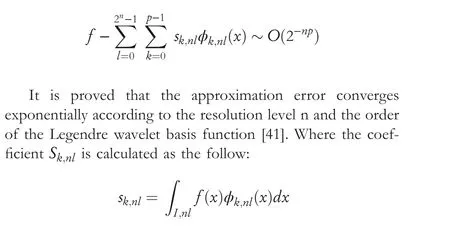
In this paper, the above coefficients are adaptively learnt during the training phase of LMWNN.
2.2 | Legendre multi‐wavelet network
The local approximation property of wavelet neurons and multiresolution learning make the WNN stronger adaptive ability,faster convergence speed,and approximation prediction ability than previous neural neurons [21, 39, 42].And LMWNN is a WNN that uses Legendre multi-wavelet as the activation function.It combines the rich properties of Legendre multi-wavelet with the self-learning, adaptive and fault-tolerance of neural networks.Typically,neural networks contain a large number of hyperparameters,and the complex process of finding the optimization needs to be done with extra algorithms in order to further improve the performance of the model[43].However,LMWNN is based on the mathematical properties of Legendre multi-wavelets, which avoids the extensive process of finding optimal parameters and reduces computational costs.Compared with other wavelet neural networks,LMWNN has a more direct and simpler network structure and a hidden layer main neuron of it is the linear combination of orthogonal explicit polynomials.These advantages can effectively decrease the number of parameters and corresponding computing costs.Furthermore,the essential attribute of the adaptive piecewise approximating enables LMWNN to locally connect and share weights involving only a subset of Legendre multi-wavelet coefficients.This local process structure effectively decreases the learning times when training.Legendre Multi-wavelet neural network has a threelayer structure with the input layer,the Legendre multi-wavelet layer, and the output layer, and its basic form is shown in Figure 2.
2.2.1 | Input layer
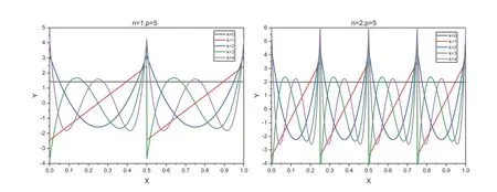
F I G U R E 1 Legendre multi-wavelet function
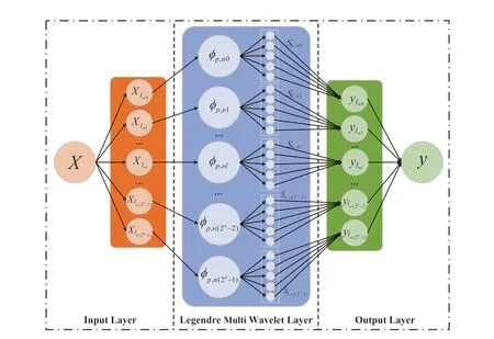
F I G U R E 2 Structure of Legendre Multi-wavelet neural network (LMWNN)
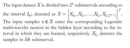
2.2.2 | Hidden layer
Each neuronφk,nlof this layer is essential for the linear combination of the dilated and translated Legendre polynomials.Each neuron containsporthogonal polynomials.In particular,the input layer and Legendre multi-wavelet layer are locally connected, and each neuron shares the weightsSk,nlThe output of thelthsubinterval of the hidden layer to the output layer is described as
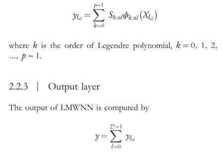
The above network structure will be used for wind speed prediction problems.
2.3 | The learning algorithm of Legendre Multi‐wavelet neural network
The learning algorithm for LMWNN is standard gradient descent algorithm.This algorithm learns Legendre multiwavelet weight coefficients between the hidden layer and the output layer in LMWNN.The objective is to minimise the loss functionEdenoted

where the update of the weight coefficients is performed according to the following learning rule:
where the number of iterationst=1, 2,...N,αis the learning rate,α>0,andmlis the number of sample points in the subinterval ofXInl.The adjustment of the network weight coefficients ends when the loss function reaches a set lower limit or the number of iterations reaches a specified value.In this process,we can also get the optimal values of the decomposition scalenand the order of Legendre multi-wavelet basisp.
2.4 | Hybrid models with Legendre Multi‐wavelet neural network
Researchers have systematically summarised and analysed the advantages of hybrid models for prediction problems [25, 44,45].Decomposition models based on a combination of signal processing techniques and machine learning methods are the popular research directions.The highly non-stationary and non-linear nature of wind speed prediction makes the predictive performance of various single models unstable due to the difficulty of a single model in learning the trends from the data.Therefore, this section describes two hybrid models based on LMWNN.
2.4.1 | EMD_LMWNN
Empirical mode decomposition is a method proposed by Nordene.Huang [46] in 1998 to deal with nonsmoothed signals,which in essence is to identify all the vibrational modes(Intrinsic Oscillatory Mode) contained in the signal by the characteristic time scale.In this process, both the typical time scale and the definition of intrinsic mode function are empirical and approximate.
The expression of the original dataX(t) decomposed by EMD is as follows:
wherecm(t)is thenth-order modal component of the original dataX(t) obtained by data processing, andrm(t) is themthorder residual obtained by subtracting the original data from themth-order modal component.
In the work of Bokde et al.[44], large numbers of decomposition models constructed based on EMD or EEMD combined with various single models are summarised,and the advantages and prospects of their application in the field of wind speed prediction are demonstrated.We construct a decomposition model to explore whether a hybrid model can improve the accuracy and performance of predictions based on a single model.The model combines EMD with LMWNN,called EMD_LMWNN.
Wavelet analysis and WNN have been widely used for wind speed prediction [23, 24].It has been shown that hybrid models obtained by combining several single models according to certain rules can effectively improve model performance[47].To explore the improvement of wind speed prediction performance by EMD, a signal processing technique, we combine LMWNN with EMD to construct a hybrid model,shown in Figure 3.
In the structure of Figure 3, EMD first decomposes the original wind speed series to obtain the component and residual components.Then, a corresponding LMWNN prediction model is built for each component.The component data are entered into the network as input sequences, and the prediction results are output after iterative computation in Legendre multi-wavelet layer.Finally, the predictions of LMWNN for each component are reconstructed to obtain the final wind speed prediction results.
2.4.2 | DWT_LMWNN
Wavelet transform, another mainstream signal processing technique, is a method for multi-resolution analysis of time series in both the time and frequency domains.Since the wind speed series are all discrete, discrete wavelets are used in the decomposition model for wind speed prediction[45].With the wavelet transform, mixed signals of different frequencies can be decomposed into sub-signals of different frequency bands,effectively dealing with problems such as signal analysis, separation of signal and noise, and feature extraction.We also construct a decomposition model to explore the performance of a hybrid model based on the combination of wavelet transform and LMWNN.Daubechies wavelets were used in combination with LMWNN, called DWT_LMWNN.
Daubechies wavelets are particularly sensitive to irregular signals and are widely used to analyse signal fluctuations.The Daubechies wavelet families [48] are discrete orthogonal wavelets designed by Daubechies,generally abbreviated asN,with N being the order of the wavelet.There are no explicit expressions fordbNwavelets, except for the db1 wavelet.Daubechies wavelets have a scale function and a wavelet function.Each layer of the scale function in multi-resolution analysis can be expressed as:
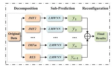
F I G U R E 3 The structure of EMD_LMWNN
wherebkis called the translation element [49].
The structure of DWT_LMWNN is shown in Figure 4.DWT_LMWNN is also a hybrid model based on a decomposition form and is treated similarly to EMD_LMWNN.Disperse wavelet transform (DWT) first decomposes the original wind speed sequence to obtain two sub-signals:approximate and detailed series [50].Then, a corresponding LMWNN prediction model is built for each sub-signal.The component data enters the network as an input sequence, and the prediction results are output after iterative computation in the Legendre multi-wavelet layer.Finally, the sub-signal predictions are superimposed to obtain the final wind speed predictions.
3 | EXPERIMENT
Based on the previously mentioned methods,LMWNN model is proposed based on Legendre multi-wavelet and validated by real wind speed datasets.In addition, to verify the superiority of its model, it is compared with three other models, BPNN,Morlet WNN, and ARIMA.Meanwhile, a fusion model EMD_LMWNN is also used as a contrast to compare with LMWNN for analysis.
3.1 | Dataset and forecast strategies
The original observations were obtained from the NREL,which involved wind sequences recorded at 5-min intervals every day from January to December 2012 at the wind speed monitoring site in Yuma, Arizona, USA.The datasets can be found at https://maps.nrel.gov/wind-prospector.The dataset 1 is selected from January-April 2012 observations,and dataset 2 is selected from July-October of the same year,which used to verify the validity and stability of the model.Depending on the time interval of the measured data(5 min,15 min,and 30 min),3600 sample points were selected as the experimental dataset,of which 3000 pieces of sample points were used as the training set, and 600 pieces of sample points were used as the prediction(test) set.As shown in Figure 5, the observed data with a time interval of 5 min are shown, the blue part is the training set, and the red part is the prediction(test) set.

F I G U R E 4 The structure of DWT_LMWNN
To further refine the experimental strategies, 3000 sample points are divided into 2992 sample groups as training sets,while 600 sample points are divided into 592 sample groups as test sets.Each group consists of an input sequence of five data and an output value.To verify the model's predictive ability at different time intervals, we recollect the data at time intervals of 5,15,and 30 min respectively.The amount of data collected each time is the same.The statistical characteristics on the wind speed sequence segments presented as line graphs in this paper is listed in Table 1.
Cross-validation is used to assess the model's stability and avoid biased results obtained by chance.In this paper draws on the recursive strategy used in the ForecastTB [13] and the rolling-origin- recalibration evaluation [51] to obtain more accurate and stable results with nested cross-validation with gaps.In addition, several experiments show that the model accuracy reaches the comprehensive optimum when the number of iterations is 1000,so the iterations is set to 1000 for all experiments in this paper.Finally, the code part of experiments in this paper are implemented by MATLAB.
To overcome the drawbacks of direct multi-step forecasting such as increased variance,and the drawbacks of recursive multistep forecasting such as error accumulation, this paper uses a method of fusing direct and recursive multi-step forecasting[52,53] to forecast wind speed.Figure 6 illustrates the prediction strategy used in this paper.First,a sequence of wind speeds from five consecutive moments is entered into the prediction model to obtain the next moment's prediction.Next,this prediction is added to the input sequence as the fifth sample data in the input sequence enters into the model to predict the next moment's result.The above steps are repeated three times to obtain the results of the three-step prediction.Then, the following five consecutive wind speed sequences enter the model,repeating to obtain a multi-step prediction model for wind speed.Each time a result is predicted,the input sequence is moved forward by one step in the forecasting process.It is known as a sliding window.The size of the sliding window in this paper is 8,meaning that the three-step prediction is performed in a sliding window.After the three prediction steps are completed in one window, the window slides down,and the prediction continues.
For sequences containing temporal information, simply splitting the dataset randomly into a training and test set using traditional cross-validation methods defies logic and can lead to data leakage and over-fitting.The time series prediction problem has a time order between sample points.Therefore,this paper designs a nested cross-validation method with gapsto verify the models.Ten randomly selected training sequences with intervals (gap) in the dataset were trained on the model,and the average of the test results of each metric was taken as the final result.

T A B L E 1 The basic characteristics in datasets

F I G U R E 5 Original wind speed datasets 1 and dataset 2.(a) dataset 1 (b) dataset 2
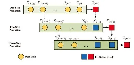
F I G U R E 6 The diagram of multi-step predicting
3.2 | Performance index
In this paper, Mean Absolute Error (MAE), Mean Absolute Percentage Error (MAPE), Root Mean Square Error (RMSE)and Mean Square Error(MSE)are used as metrics to evaluate the validity of these models.Root Mean Square Error measures the deviation between the predicted and actual values, and a more considerable RMSE value indicates a more significant error.Mean Absolute Error measures the MAE between the predicted and actual values,with a more petite MAE indicating a better model.Mean Absolute Percentage Error is also a measure of prediction accuracy.The coefficient of determination describes whether the predicted value is linearly related to the actual value and ranges from 0 to 1.The larger the R-Squared,the better the predicted value explains the actual value.
where ︿yidenotes the predicted value,yidenotes the actual value,yidenotes the average of the actual values, andNdenotes the number of samples.In addition,the improved RMSE(PRMSE) performance is used as a measure of the improvement of the model compared to the benchmark models.
whereRMSE1denotes the RMSE obtained from the proposed model experiments, andRMSE2denotes the RMSE obtained from the contrast models experiments.
3.3 | Wind power forecasting analysis
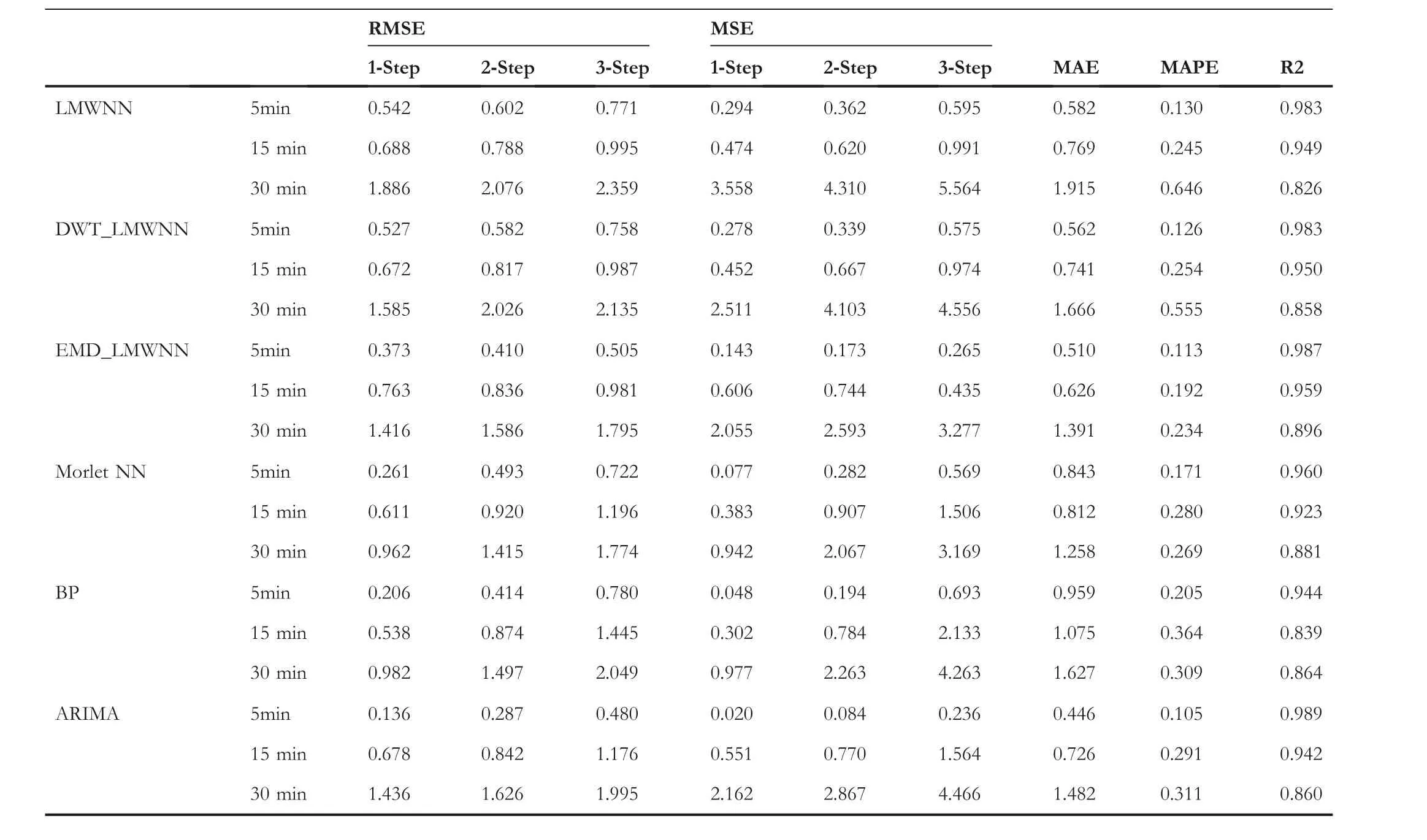
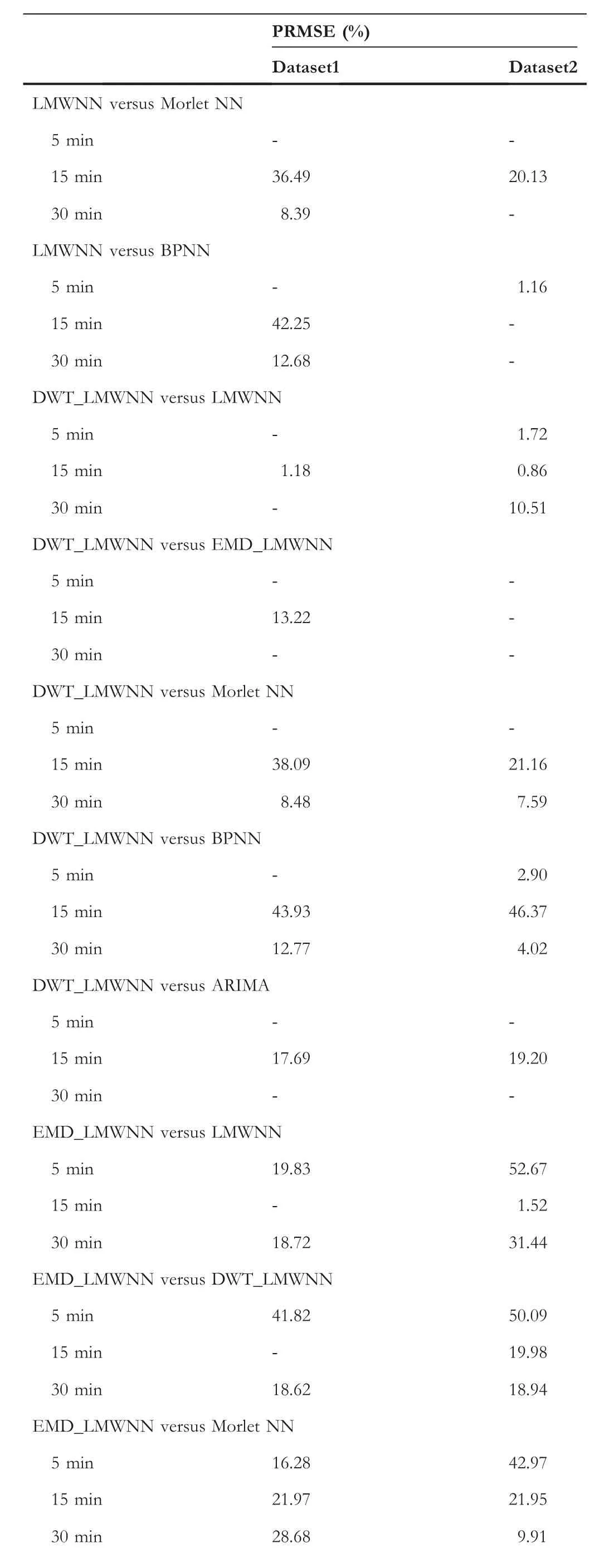
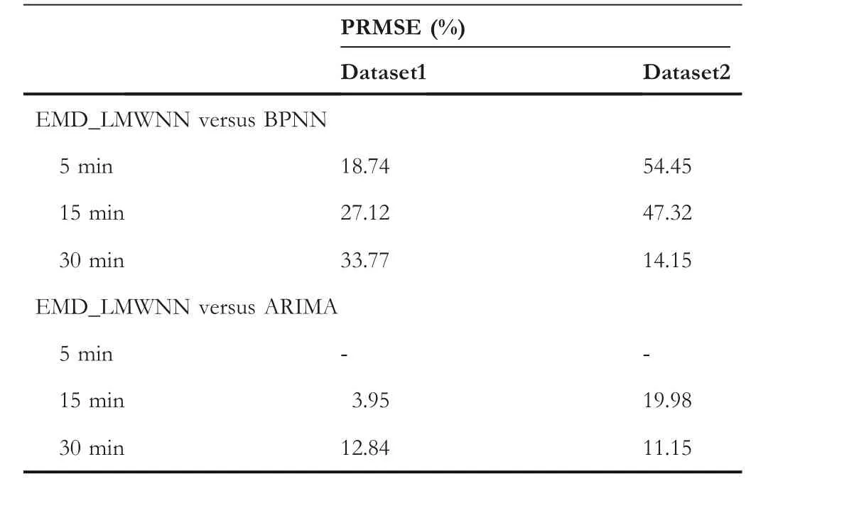
To verify the effectiveness of LMWNN,a comparative analysis of the proposed model with three other representative prediction models,namely Morlet WNN,BP neural network,and ARIMA, are performed.In addition, a hybrid model EMD_LMWNN combined with EMD and a hybrid model DWT_LMWNN combined with DWT were also built to explore whether the hybrid model would improve the prediction performance.Tables 2 and 3 show the values of the five metrics obtained in the experiments for the models mentioned above.Table 4 records the improvement in RMSE scores for the proposed model versus the other models for the three-step predictions.It is important to note that if there is no improvement in RMSE scores, the corresponding position in the table is filled with a short horizontal line to indicate no improvement in RMSE scores.
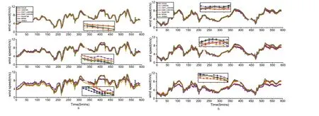
Figures 7, 8, 9 show a comparison of the one-step, twostep, and three-step prediction results on the two datasets.(In these figures, (a) shows results on dataset 1 and (b) shows results on dataset 2).To verify the improvement in computational speed by LMWNN, the training time for each model is recorded in Table 5.The effective and efficient properties of LMWNN are corroborated by comparing the training times of the different models.Figure 11 shows the single-step prediction results for LMWNN, DWT_LMWNN and EMD_LMWNN models on two datasets.It should be mentioned that there are 5, 15 and 30 min time intervals of the datasets collection in all the experiment.
It is evident from Tables 2 and 3 that the proposed prediction model has significant advantages in all evaluation metrics, especially the single-step prediction.For dataset 1, its RMSE values for single-step prediction at 5-min time intervals is 0.066, which improves the prediction accuracy by 87.87%over EMD_LMWNN's, 73.28% over Morlet-NN's, 59.76%over BPNN's, and 37.74% over ARIMA's.For dataset 2, its RMSE values for single-step prediction at 5-min time intervals is 0.063, which is 86.96% better than the RMSE of EMD_LMWNN, 82.74% better than Morlet-NN, 77.97%better than BPNN,and 54.68%better than the ARIMA model.
3.3.1 | Comparison of different models
To discuss the predictive performance of the LMWNN model and its hybrid models combined with signal processingtechniques, this section compares the proposed model with earlier proposed models,including the Morlet NN,BPNN and the differential AR sliding average model (ARIMA).Specifically, BPNN and ARIMA models are commonly used as benchmarks for short-term wind speed prediction.In addition,Morlet NN is a compact WNN combining wavelet basis functions with neural networks, which is widely used for forecasting.Tables 2 and 3 show a comparison of the scores of the evaluation for the different models on the two datasets.Table 6 shows the average scores of the evaluation for the proposed model and the predicted results of the earlier model on the two datasets.Figures 7, 8, 9 compare the linear representations of the single-step and multi-step prediction results for all models for the three time intervals.
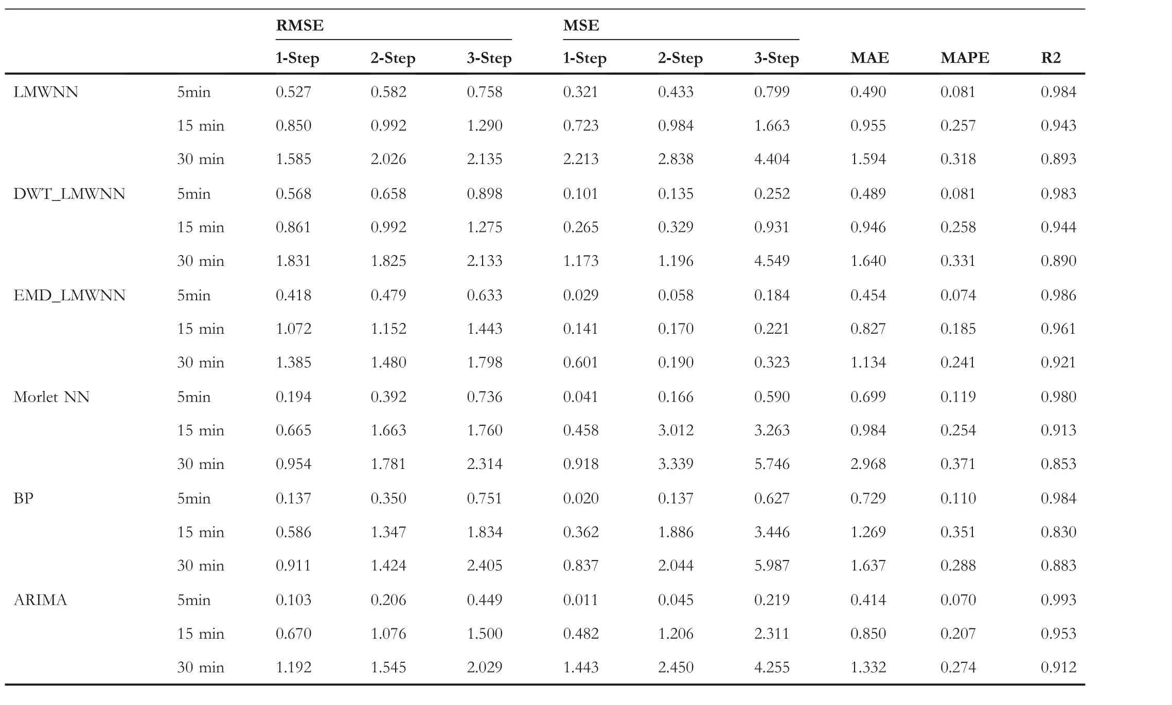
T A B L E 2 The prediction error with various models on Dataset1
T A B L E 3 The prediction error with various models on Dataset2
T A B L E 4 The improvements between the proposed model and other models
TA B L E 4 (Continued)
Legendre Multi-wavelet neural network was successfully applied to wind speed prediction.As shown in Tables 2 and 3 the proposed prediction models have significant advantages in evaluation metrics, especially when the wind speed unsteadiness increases.Table 6 shows that the average RMSEs of LMWNN for one-step,two-steps and three-step predictions at 5 min time interval are 0.065, 0.075 and 0.086, at 15 min time interval are 0.080,0.093 and 0.108,at 30 min time interval are 0.097, 0.110 and 0.122.Compared to the corresponding metrics of all other models, LMWNN obtains the smallest error values.In addition, the PRMSEs in Table 6 shows that the average RMSE scores of DWT_LMWNN's one-step,two-step and three-step predictions are 0.766,0.904 and 1.131 at 15 min time interval, respectively.While at 30 min time interval, the average RMSE scores of EMD_LMWNN's one-step,two-step and three-step predictions are 1.400, 1.533 and 1.796, respectively.The hybrid model based on LMWNN obtained the smallest error values compared to the corresponding metrics of all other models.In addition, LMWNN's RMSE scores for one-step, two-step and three-step predictions are 0.769, 0.890 and 1.142 at 15 min time interval, respectively.LMWNN's RMSE scores for one-step,two-step and three-step predictions are 1.736,2.051 and 2.247 at 30 min time interval,respectively.Compared with the other two hybrid LMWNN-based models,the hybrid model combining LMWNN and signal processing techniques have significantly improved the prediction accuracy over the single model.The experimental results validate the positive impact of the decomposition techniques (EMD and DWT)on the wind speed prediction problem and illustrate the effectiveness of the proposed EMD_LMWNN and DWT_LMWNN for the prediction problem.The hybrid model based on LMWNN has similar advantages to previously studied hybrid models for wind speed prediction.
F I G U R E 7 Multi-step wind speed forecast results by different models for datasets (5 min).(a) dataset 1 (b) dataset 2
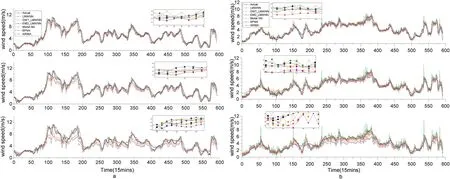
F I G U R E 8 Multi-step wind speed forecast results by different models for datasets (15 min).(a) dataset 1 (b) dataset 2
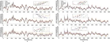
F I G U R E 9 Multi-step wind speed forecast results by different models for datasets (30 min).(a) dataset 1 (b) dataset 2
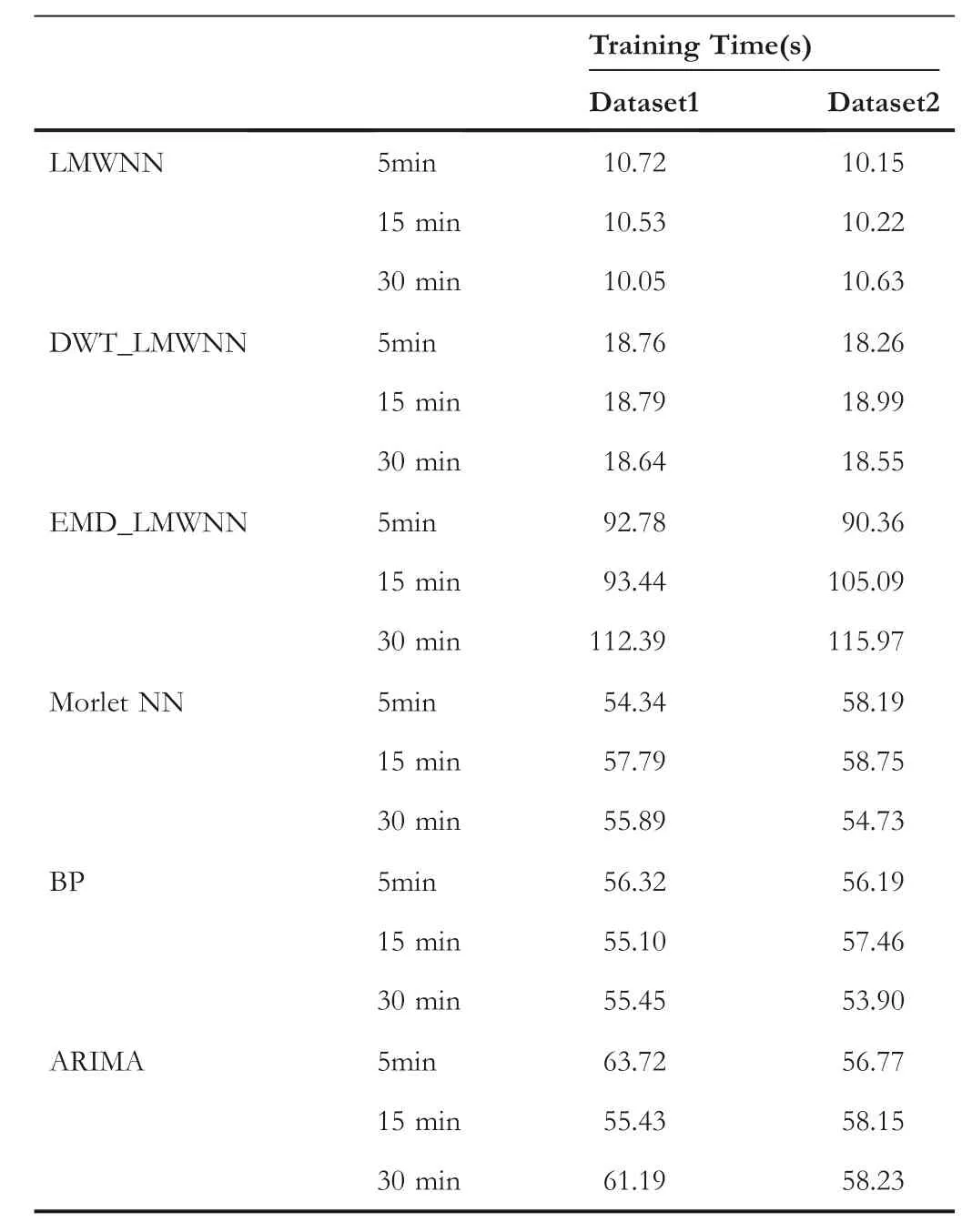
T A B L E 5 Training time for different models on two datasets
It is well known that Morlet NN and BPNN are traditional and widely used neural networks in prediction problems.As shown in Table 4,a comparison of LMWNN with Morlet NN and BPNN shows that LMWNN outperforms the latter in terms of predictive power.For example, LMWNN's RMSE scores on both datasets are 36.49% and 20.13% lower than those of Morlet NN and 42.25% lower than those of BPNN for a 15 min time interval.Because of the increased unsteadiness of the wind speed due to the increased sampling interval,the prediction accuracy decreases.However, in this case,LMWNN still scores 8.39% lower than the RMSE of Morlet NN and 12.68% lower than the RMSE of BPNN.That is a good indication of the potential for LMWNN to excel in prediction problems.We can also say that the Legendre multiwavelet makes sense as an activation function for neural networks.
Furthermore, the PRMSEs in Table 4 show that both DWT_LMWNN and EMD_LMWNN demonstrate some advantage in their predictive ability at different time intervals.For example, in dataset 2, the PRMSE score of EMD_LMWNN compared with BPNN at 5 min time intervalis 54.45, meaning that EMD_LMWNN's RMSE score is 54.45% lower than the RMSE score of BPNN.The table shows that although the hybrid models proposed in this paper can perform wind speed prediction with high accuracy,they do not perform well at 5 min time interval.DWT_LMWNN, in particular, can only slightly reduce the prediction error based on the traditional model.However,it is worth mentioning that DWT_LMWNN's PRMSE score is generally higher than that of BPNN at 15 min interval, with the highest score reaching 46.37.That means that the prediction error obtained by DWT_LMWNN at 15 min interval is 46.37% lower than that of BPNN.That indicates to some extent that DWT_LMWNN can also achieve good prediction results with high unsteadiness sequences.Furthermore, compared with the single LMWNN,the hybrid model combining DWT and EMD can optimise further improvement in the prediction performance of the single model.It again demonstrates hybrid models'advantages and validates the positive role of signal processing techniques in hybrid models.
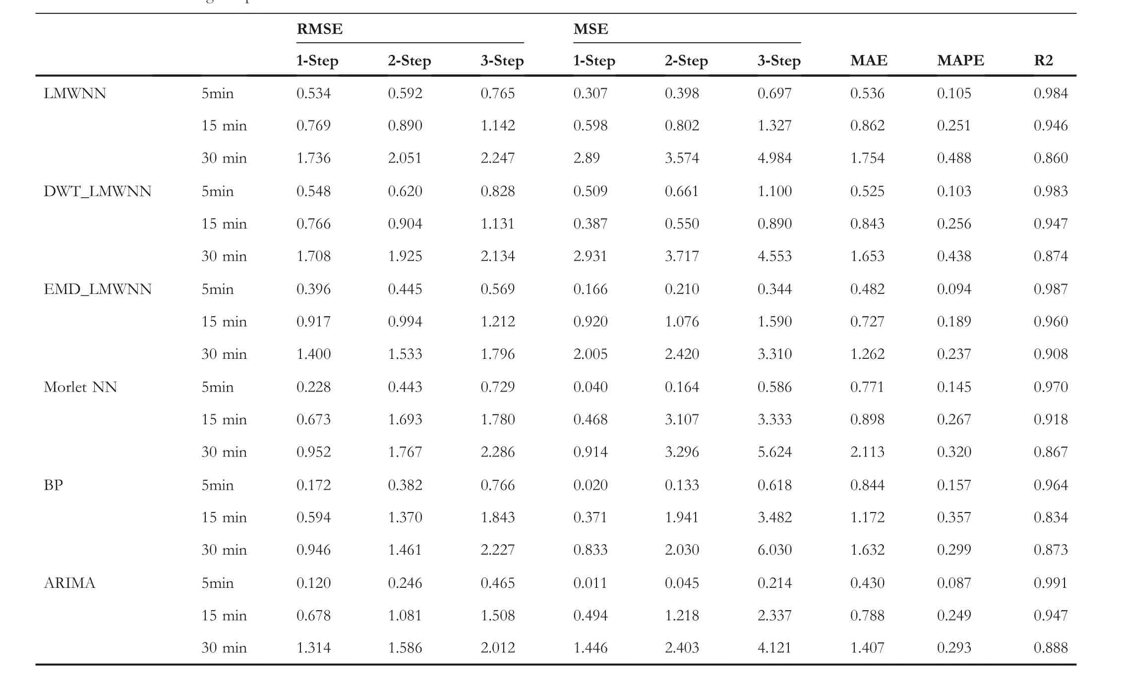
T A B L E 6 The average of prediction error with various models on two datasets
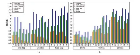
F I G U R E 1 0 Histogram of the predicted Root Mean Square Error (RMSE) of the proposed model and the earlier prediction models.(a) Histogram of RMSE values at different prediction steps.(b) Histogram of RMSE values at different sampling intervals
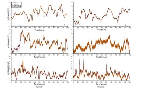
F I G U R E 1 1 Single-step wind speed forecast results by Legendre Multi-wavelet neural network (LMWNN)and EMD_LMWNN models for datasets.(a)forecasting result in dataset 1 at 5 min interval.(b) forecasting result in dataset 2 at 5 min interval.(c) forecasting result in dataset 1 at 15 min interval.(d)forecasting result in dataset 2 at 15 min interval.(e) forecasting result in dataset 1 at 30 min interval.f forecasting result in dataset 2 at 30 min interval
Analysing combined Tables 2–4 and 6, the prediction performance of EMD_LMWNN is the most effective of all the models.At 15 min time interval, EMD_LMWNN's MAE in dataset1 for three-step prediction is 0.827, the MAPE is 0.185, and the R-square score is 0.961.At the 30 min time interval, EMD_LMWNN's MAE in dataset1 for three-step prediction is 1.134, the MAPE is 0.241, and the R-square score is 0.92.At 15 min time interval, EMD_LMWNN's MAE in dataset2 for three-step prediction is 0.626,the MAPE is 0.192, and the R-square score is 0.959.At 30 min time interval, EMD_LMWNN's MAE in dataset2 for three-step prediction is 1.391, the MAPE is 0.234, and the R-square score is 0.896.We can also find the excellent predictive power of ARIMA for smoother series.Autoregressive integrated moving average has the highest evaluation score at the 5 min time interval.However, the volatility of wind increases with increasing time intervals and forecast steps.The predictive ability of ARIMA decreases as the instability of wind increases,indicating that ARIMA is not an optimal solution to the sequence prediction with high unsteadiness.Comparing the prediction results of ARIMA and EMD_LMWNN shows the excellent prediction ability of EMD_LMWNN for sequences with high non-stationarity.Also, it shows that EMD_LMWNN is suitable for dealing with highly nonstationarity prediction problems.
As shown in Figure 10a is the average prediction RMSEs of the five models at multi-step prediction on two datasets.The orange bars indicate the RMSEs at 5 min time interval,the green bars indicate the RMSEs at 15 min time interval,and the blue bars indicate the RMSEs at 30 min time interval.Figure 10b shows the aver-age prediction RMSEs of these five models at three time intervals.The orange bars indicate the RMSEs for single-step prediction, the green bars indicate the RMSEs for two-step prediction,and the blue bars indicate the RMSEs for three-step prediction.According to Figure 10a,it can be found that the RMSEs of the prediction results are on an increasing trend as the prediction step size increases.According to Figure 10b, it can be found that the RMSEs of the prediction results are also on an increasing trend as the sampling time interval increases.Additionally, we can find a significant advantage in the RMSE scores of ARIMA single-step predictions at 5 min time interval.However, the decrease in predictive ability is most pronounced as the prediction step and sampling time interval increase,indicating that ARIMA cannot cope effectively with fluctuating wind speed forecasts and that the model has poor generalisation capability.In contrast,LMWNN-based models can handle the situation better.The trend of prediction error is more stable when the wind speed volatility increases, indicating that the LMWNN-based wind speed prediction methods have stronger robustness and more stable prediction capability.Combining these two charts, we can further find that the effect of increasing the sampling time interval on the prediction results will be greater than increasing the prediction step size on the prediction results.Because the prediction RMSEs of the 30 min time interval in the same prediction step in Figure 10a are steeply higher, while the RMSEs of the three-steps prediction in the same time interval in Figure 10b are not significantly larger than the RMSEs of the two-steps prediction.
Numerous experimental comparisons show that when the number of iterations of the Morlet WNN and BPNN increases, their prediction accuracy improves is further improved, but their running time also increases.While at the same 1000 iterations, LMWNN and its hybrid models can achieve satisfactory accuracy.In comparison, the traditional time series forecasting model ARIMA can cope well with relatively smooth situations.(nevertheless, its forecasting accuracy is still lower than that of the LMWNN model.) When the time interval and forecasting step size increase and the data instability increases, the forecasting performance of the ARIMA model decreases rapidly.However, the appropriate prediction step size for statistical models is usually 3–5 steps,so the prediction results of 1–2 steps can only be used as an experimental comparison to verify the model performance and cannot be used for applications.The performance metrics of model prediction are shown in Tables 2 to 4.
By comparing the performance metrics with different prediction steps horizontally and then comparing the performance indexes of different models vertically, it becomes clear that every model's prediction accuracy falls as the number of prediction steps increases.In multi-step forecasting, the ARIMA model, which effectively deals with linear issues, has the most apparent decline in prediction accuracy,suggesting its inability to cope with non-stationary data.It is not good at dealing with prediction problems with intermit-tent and stochastic characteristics, such as wind speed.In contrast, the LMWNN proposed in this paper not only achieves better prediction capability, but its hybrid model combined with EMD also yields optimal prediction results in high non-stationarity wind speed prediction.Through experiments on different data sets, different time intervals, and different prediction steps, it is demonstrated that EMD_LMWNN can satisfactorily result in more accurate and reduce the forecast inaccuracy of wind speed.
The difficulty with wind speed prediction is the excessive volatility — the part of the wind speed that suddenly rises or falls is difficult to predict accurately.The wind speed multi-step prediction results are shown in Figures 7,8,9.We can find that when the time interval increases and the correlation of wind speed at each moment weakens, its uncertainty rises, resulting in its prediction at each moment without high accuracy.As shown in Figure 7, the wind speed peaks that are reached abruptly are challenging to predict accurately in the prediction.In addition, the results of two-step and three-step prediction under the condition of a 15-min interval exhibit relatively large inaccuracies, as shown in Figure 8, especially for models like ARIMA that are applicable to smooth data.Nevertheless, the EMD_LMWNN model proposed in this paper still maintains a low error value compared with other earlier models.
3.3.2 | Comparison of models' training time
It is noteworthy that LMWNN significantly reduces the training time of the models.All comparison experiments were performed at the same time interval and the models were trained in the same way (both data divisions and number of iterations are the same).The training times for different models at different time intervals are shown in Table 5.On both datasets, the LMWNN model has the shortest training time.As the experiment results on Dataset1, the LMWNN training time is 10.72s for a 5-min time interval,it is 10.53s for a 15-min time interval and 10.05s for a 30-min time interval.Thus, the model training time is independent of the volatility of the dataset.
In contrast, the training times for other single models at the same time interval almost always reach around 60s.At 5 min time interval, the training time of BPNN is 56.10s, the training time of Morlet NN is 58.19s and the training time of ARIMA is 56.77s.The computational speed of LMWNN is improved by more than 5 times compared to other single models.The reason for the significant reduction in training time is the main neurons in the hidden layer of LMWNN are linear combinations of orthogonal polynomials, rather than derivatives of traditional sigmoid or Gaussian-type activation functions.It can effectively reduce the number of parameters and the corresponding computing costs.
As a hybrid model, DWT_LMWNN has a significant advantage in terms of training time.Although DWT_LMWNN is a combination of DWT with a single model,the training time does not change much.DWT_LMWNN's training time is 18.76s at 5 min time interval,18.79s at 15 min time interval and 18.64s at 30 min time interval.However, the training time for EMD_LMWNN is much longer.The training time of EMD_LMWNN is 92.78s at 5 min time interval.As the sampling time interval increases,the sequence non-stationarity increases and the complexity of the modal decomposition increases,which further increases the training time of the model,with the training time of EMD_LMWNN at 15 min time interval is 93.44s and the training time is 112.39s at 30 min time interval.It demonstrates that hybrid models tend to take longer to train than single models, and brings up a discussion as whether the improvement in prediction accuracy is worth the sacrifice in computational time at this situation.Considering the previously mentioned prediction performance,as shown in Tables 2 to 4, it can be found that EMD_LMWNN sacrifices training time for optimal prediction capability.
3.3.3 | Comparison of single-step predictions
To further discuss the prediction performance of LMWNN and its hybrid models, an experimental comparison of LMWNN,DWT_LMWNN and EMD_LMWNN for single-step prediction is also conducted in this paper.The two hybrid models mentioned in this paper are based on a decompositionreconstruction frame of the hybrid model.Empirical mode decomposition or DWT first decomposes the wind speed sequences.Then LMWNN performs subseries fitting and finally reconstructs to obtain the predicted values.For dataset 1 and dataset 2, Figure 11 shows the linear representations of the single-step prediction results for the two models for time intervals of 5, 15, and 30 min.The significant difference in prediction accuracy on different data sets at different time intervals is due to the different standard deviations of the data in the test sets at different time intervals.A more significant standard deviation of the sequences indicates higher non-stationarity of the data observations.The fitting of the predictions to the actual data decreases as the non-stationarity rises with increasing time intervals.In both cases (dataset 1 and dataset 2), the model prediction accuracy decreases as the data sampling interval increases.Figure 11a,b shows visually that all three models fit satisfactorily at 5 min time interval.However,as seen from the green wireframe markers in Figure 11, the EMD_LMWNN forecasts appear anomalous when the wind speed trend changes.This problem is caused by high-frequency signals with small amplitude at a certain moment or minimum time interval during the decomposition process, resulting in mode mixing[46].EMD_LMWNN has some points with significant prediction errors due to pattern mixing and requires extra processing time for data decomposition and reconstruction.It also explains the particularly long training time of EMD_LMWNN.Despite the occasional large fluctuations, the predictive power of EMD_LMWNN is still superior.
As shown in Figure 11c–f, DWT_LMWNN does not handle sudden increases and decreases in wind speed at the adjacent moment points well, and the predictive capability decreases faster than EMD_LMWNN.As seen from the purple wireframe markings in Figure 11, there is nothing DWT_LMWNN can do when the sequence fluctuates sharply.Since DWT_LMWNN lacks adaptivity,the mother wavelet and its parameters(stretch and translation factors)must be manually selected.When the wavelet basis and scale functions used to decompose a sequence are selected,it may be the case that they cannot be applied to different sequences.In general, DWT decomposes a complex wind speed sequence to obtain a relatively smooth subsequence and then learns its features through the excellent fitting ability of LMWNN.Once the decomposition operation cannot be applied to the current series,however,the predictive power of the hybrid model becomes less satisfactory.If it is desired DWT_LMWNN to get better prediction ability, selecting the parameters and mother wavelet would require more labour costs.It conflicts with wind speed's variable and stochastic nature and proves that EMD_LMWNN is the superior hybrid model for forecasting.
4 | CONCLUSION
To explore the application of the model combining the Legendre multi-wavelet function and neural network in prediction problems,we propose a compact WNN LMWNN.Based on the selflearning ability of the neural network,the appropriate Legendre multi-wavelet basis can be found in training phase,and avoids the complex calculation of parameters selection of WNN.While traditional models are prone to overfitting and optimum local problems,the LMWNN is adaptively trained to fit and has better predictive ability than other traditional neural networks,reflecting its significance and merits.It is sufficient to demonstrate that the attempt to use Legendre multi-wavelets as an activation function is successful and meaningful.Moreover,LMWNN can reduce the computing costs and computing time because the main neurons in the hidden layer are linear combinations of orthogonal polynomials.The experimental results show that the training time of LMWNN is much faster than that of other neural network models, which also provides a new research direction for optimising large-scale data training in the future.Given the various advantages of hybrid models in wind speed prediction, we also tried the hybrid models EMD_LMWNN and DWT_LMWNN in combination with signal processing techniques.Both signal processing techniques are beneficial in improving the performance of wind speed prediction.EMD_LMWNN and DWT_LMWNN both optimise the prediction accuracy based on LMWNN.However,the performance of DWT_LMWNN is not satisfactory since DWT is a signal processing method that lacks adaptivity and is not well suited to variable and highly stochastic wind speed series.Therefore,it can be said that it is not always possible to improve prediction performance by stacking multiple models.The combined evaluation metrics show that EMD_LMWNN achieves optimal results in wind speed prediction,reducing the error in wind speed prediction and improving the prediction results.However, the decomposition and reconstruction process of EMD is time-consuming,so improving the self-adaptiveness of the hybrid model and optimising the training speed can be a more in-depth research direction in the future.
ACKNOWLEDGEMENTS
This work is funded by Fundamental and Advanced Research Project of Chongqing CSTC of China (No.cstc2019jcyjmsxmX0386 and No.cstc2020jcyj-msxmX0232) and National Statistical Science Research Project (No.2020LY100).Moreover,the authors wish to thank the people who have helped in this study, but whose names are not listed in the paper.
CONFLICT OF INTEREST
None.
DATA AVAILABILITY STATEMENT
These data were derived from the following resources available in the public domain: https://maps.nrel.gov/wind-prospector/?aL=kWBYWk%255Bv%255D%3Dt&bL=clig ht&cE=0&lR=0&mC=40.212440718286 466%2C-91.58203125&zL=4.
ORCID
Dongqing Jiahttps://orcid.org/0000-0001-9028-0533
 CAAI Transactions on Intelligence Technology2023年3期
- CAAI Transactions on Intelligence Technology的其它文章
- Fault diagnosis of rolling bearings with noise signal based on modified kernel principal component analysis and DC-ResNet
- Anti‐noise diesel engine misfire diagnosis using a multi‐scale CNN‐LSTM neural network with denoising module
- Iteration dependent interval based open‐closed‐loop iterative learning control for time varying systems with vector relative degree
- Thermoelectric energy harvesting for internet of things devices using machine learning: A review
- An embedded vertical‐federated feature selection algorithm based on particle swarm optimisation
- An activated variable parameter gradient-based neural network for time-variant constrained quadratic programming and its applications
