Multi-Scale Neural Networks Based on Runge-Kutta Method for Solving Unsteady Partial Differential Equations*
CHEN Zebin,FENG Xinlong
(School of Mathematics and System Sciences,Xinjiang University,Urumqi Xinjiang 830017,China)
Abstract: This paper proposes the multi-scale neural networks method based on Runge-Kutta to solve unsteady partial differential equations.The method uses q-order Runge-Kutta to construct the time iteratione scheme, and further establishes the total loss function of multiple time steps,which is to realize the parameter sharing of neural networks with multiple time steps,and to predict the function value at any moment in the time domain.Besides, the m-scaling factor is adopted to speed up the convergence of the loss function and improve the accuracy of the numerical solution.Finally,several numerical experiments are presented to demonstrate the effectiveness of the proposed method.
Key words: unsteady partial differential equations;q-order Runge-Kutta method;multi-scale neural networks;m-scaling factor;high accuracy
0 Introduction
Deep learning has achieved satisfactory results in searching technology,natural language processing,image processing,recommendation system, personalization technology, etc.In recent years, deep learning has been successfully applied to solve partial differential equations and has been deeply promoted.Compared with the finite element method[1]and the finite difference method[2],deep learning as a meshless method,can mitigate the curse of dimensionality when solving highdimensional partial differential equations.So it is more convenient to establish a solution framework for high-dimensional partial differential equations.E etc[3]proposed the Deep-Ritz method based on deep neural networks for numerically solving variational problems,which was insensitive to the dimension of the problem and could be used to solve high-dimensional problems.Physics-Informed Neural Networks(PINNs)[4]used the automatic differentiation technique[5]for the first time to embed the residual of the equation into the loss function of the neural networks,and obtained the numerical solution of the equation by minimizing the loss function.PINNs is a new numerical method for solving partial differential equations,which makes full use of the physical information contained in the PDEs.PINNs have attracted the attention of many scholars,and literature[6-7]shows theoretical convergence of PINNs for certain classes of PDEs.Multi-scale DNN[8]proposed the idea of radial scaling in the frequency domain,which had the ability to approximate high-frequency and high-dimensional functions,and could accelerate the convergence speed of the loss function.
Recently,the research on deep learning algorithms for nonlinear unsteady partial differential equations have attracted the attention of many scholars.The time-discrete model of PINNs can still guarantee the stability and high precision of numerical solutions when using large time steps, but it needs high computational costs.DeLISA added the physical information of the governing equations into the time iteration scheme, and introduced time-dependent input to achieve continuous-time prediction without a large number of interior points[9].On this basis, this paper proposes a multi-scale neural networks algorithm integrating Runge-Kutta method.On the one hand, the algorithm constructs a time iteration scheme to build the total loss function of multiple time steps, thus realizes the sharing of neural networks parameters in multiple time steps to save computational costs.It can also predict the function value at any time in the time domain after training.On the other hand,the algorithm can not only speed up the convergence speed of the loss function,but also improve the accuracy of the solution.In the numerical example, we compare the stability of the time stepping scheme and the time iteration scheme in multi-time-step solutions.Then, through the sensitivity analysis of boundary points and initial points, we find that the solution accuracy does not increase with the increase of points.Therefore,we can still achieve the same calculation accuracy by selecting an appropriately small number of points,and achieving the purpose of reducing the amount of calculation.
The rest of this paper is organized as follows: In section 1, we describe neural networks combined with Runge-Kutta method and automatic differentiation in detail.Section 2 shows time iteration scheme based on Runge-Kutta multi-scale neural networks.We then present several numerical experiments, including Convection-Diffusion equation and Burgers equation in section 3.Finally,we conclude with the key ideas raised in this work.
1 Preliminaries
In this section, we introduce the neural networks integrates the Runge-Kutta[10]method to solve unsteady partial differential equations in detail.Automatic differentiation is briefly introduced, and the computational steps of the automatic differentiation are understood by calculating the derivatives of the output of a simple structured neural networks with respect to the input.
1.1 Fusion of Neural Networks and Runge-Kutta Method
To understand the key idea clearly,we consider a class of unsteady partial differential equations defined on the bounded set Ω ?Rn
where x ∈Ω represents the space vector, and N represents the differential operator with respect to function u.We give the space discrete of equation(1),and then integrate it in the interval[tn,tn+1]to get
where tn=nΔt.We use the q-order implicit Runge-Kutta method to approximate the right-hand integral term in the above equation
where un+ci(x)=u(tn+ciΔt,x),0 <aij,bj,cj<1.As shown in Fig 1,we give the fusion frame diagram of the neural networks and the Runge-Kutta method when x=(x1,x2)∈R2, q=5.
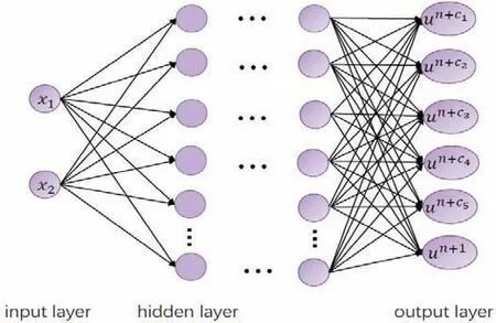
Fig 1 Fusion frame diagram of neural networks and Runge-Kutta method
From equation(2),we could include the indirect label of the output layer of the neural networks
In the following,we establish the loss function for the n-th time layer
where un(xk)is the known function value of the n time step.Similarly,we set the loss function on the boundary
where un+cq+1=un+1.Then the total loss function of equation(1)consists of the above two parts
1.2 Automatic Differentiation
PINNs embed the residual of the equation into the loss function of the neural networks for the first time,which provided an effective means to numerically solve partial differential equations.By calculating the derivative of the networks output with respect to the input,we can obtain the residuals of the equation.The numerical solution uANNconstructed by the neural networks have a specific functional expression, so the derivative can be calculated using finite difference method, symbolic differentiation or automatic differentiation.However, the limitations of the finite difference method lie in truncation error and method error.Symbolic differentiation is computationally expensive and time-consuming.Automatic differentiation can overcome the limitations of the above two methods,so this paper uses the automatic differentiation technique to calculate the derivative.
Automatic differentiation(AD) computes derivatives using the chain rule.AD calculation process can be divided into two steps: calculating the function value in the forward mode and calculating the derivative value in the reverse mode.We learn about AD by computing the derivative of the output of a multi-layer feedforward neural networks with respect to the input.The neural networks consists of an input layer with two neurons x1and x2, a hidden layer with one neuron and an output layer with one neuron y.
The calculation of the derivative of y with respect to(x1,x2)at(2,3)is shown in Table 1.

Table 1 Automatic differentiation technique derivation process
Iri etc[11]give the proof of the computational complexity of AD which proves that the computation of the gradient is at most 5 times that of the function, regardless of the dimension of the independent variable.For an optimization problem with a 100-dimensional smooth objective function, we use symbolic differentiation or numerical differentiation to compute the gradient, and then the gradient is at least 100 times more computable than the function value, not to mention the use of second-order derivative information or higher-dimensional functions.If AD is used, regardless of the dimension of the independent variable,the computation amount of the gradient is at most 4 times than the value of the function with machine precision.
2 Multi-Scale Neural Networks Integrating Runge-Kutta Method
According to the universal approximation theorem[12], as long as a hidden layer contains enough neurons, the neural networks can approximate a continuous function defined on a compact set with arbitrary accuracy.It should be noted that the neural networks obeys the frequency principle[13]when fitting the function: it tends to preferentially fit the low-frequency part of the objective function.Based on the understanding of the frequency principle, in order to solve the characteristics of slow learning at high-frequency, we can make some special designs for the neural networks.From the point of view of function space, the basis function of neural networks is composed of activation functions.The basis functions of different scales construct a feasible function space,which can approximate the objective function faster.The same basis function can be scaled to generate different scales basis functions.In order to describe the multi-scale neural network conveniently, we only divide the neurons into h parts in the first hidden layer, as shown in Fig 2.The input of the i-th neuron is ix, and the corresponding output is σ(iwx+b).Then the multi-scale neural network with L-1 hidden layers is defined as
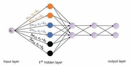
Fig 2 Multi-scale neural network example of h=3
where ⊙is the Hadamard product,m-scaling factor is M=m×(1,1,···,1,2,···,2,···i,···,i,···,h,···,h).
The m-scaling factor of multi-scale neural networks can not only speed up the convergence speed of the loss function,but also improve the accuracy of the solution.In Fig 3, we present a schematic diagram of the framework of time iteration scheme based on multi-scale neural networks.The input-output mapping of a multi-scale neural network is
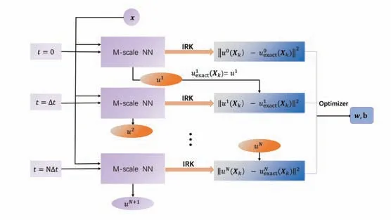
Fig 3 Time iteration scheme of neural networks combined with Runge-Kutta method
In Fig 4,we give a schematic diagram of the time step scheme of the neural networks and implicit Runge-Kutta(IRK)fusion.It is worth noting that the iterative solution of each time step in this framework requires a neural network to fit.The iterative solution of multiple time steps needs to optimize the parameters of multiple neural networks.Time iteration scheme makes full use of the approximation ability of the neural networks by adjusting the input-output mapping relationship of the multi-scale neural networks,so that the iterative solutions of multiple time steps share the parameters.At n-th time step,we set the loss function as follows
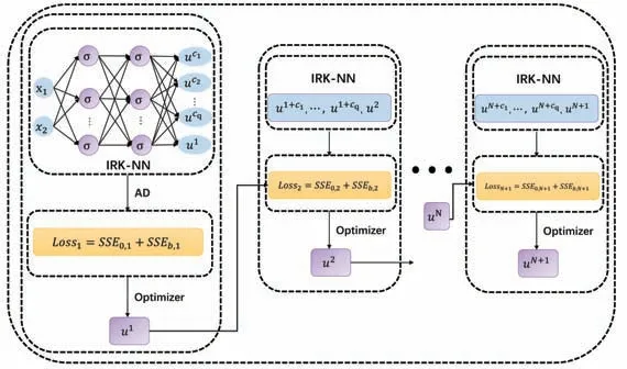
Fig 4 Time stepping scheme of neural networks combined with implicit Runge-Kutta method
We set the loss function for boundary conditions as follows
Similarly,we set the loss function for the initial condition as follows
So the total loss function can be written as
The multi-scale neural networks algorithm incorporating the Runge-Kutta method requires only a small number of initial value data pairs,constructs its time iteration scheme by IRK method,and then builds the total loss function for multiple time steps to obtain the function value at any time in the time domain by only one time optimization.
3 Numerical Experiments
In this section, in order to verify the effectiveness of the time iteration scheme algorithm based on multi-scale neural networks,we give numerical experiments to solve the Convection-Diffusion equation and Burgers equation respectively,and define the relative L2error as
3.1 Convection-Diffusion Equation
Convection-Diffusion equation[14]is widely used to describe fluid models and many physical phenomena.The unknown function u can be used to express the contaminant concentration transported through the fluid.Of course, it can also be expressed as the temperature of the fluid moving along the hot wall or the electron concentration in a semiconductor device model.To verify the stability of time iteration scheme,let’s consider a two-dimensional Convection-Diffusion equation.
where the solution area of the equation is defined as Ω=[-1,3]2,T=1,and β=(a,b).The initial boundary value conditions for this problem are given by the following true solutions
where a=b=4/5.Specifically we choose 5 hidden layers neural network with 60 neurons in each hidden layer,and tanh as activation function.The training set is composed of N0=16×16 initial value condition data pairs and Nb=50×4 boundary points data pairs.We use implicit Runge-Kutta method with q=4, and take the time step Δt=0.2.After establishing the loss function through time iteration scheme, we employ the L-BFGS-B algorithm to optimize.In Table 2, we apply time step scheme(TSS) and time iteration scheme(TIS) to solve the Convection-Diffusion equation, respectively, and then give a comparison of the relative L2error at different times by strictly controlling the variables.Compared with the traditional discrete method,the relative L2error of the TSS numerical solution method increases with the iteration of the time step.The numerical accuracy of the iterative solution of TIS at multiple time steps is significantly better than that of TTS.

Table 2 Comparison of the relative L2 error of TSS and TIS in solving the Convection-Diffusion equation at different times
3.2 2D Burgers Equation
Burgers equation is a kind of basic partial differential equation that often appears in many fields of applied mathematics.It is widely used in fluid mechanics, nonlinear acoustics, aerodynamics and traffic flow.It is the result of the combination of nonlinear waves and linear diffusions and is the simplest model to analyze the combined effects of linear advection and diffusion.Next,we consider the following two-dimensional Burgers equation[15]to compare the difference in the convergence speed and solution accuracy of the loss function using a multi-scale neural network and a fully connected neural network.
where β = (u(x,y),1)T, Ω = [0,1]×[0,1], and T = 2.The initial boundary value condition of equation (4) is given by the following analytical solution
In this example,the multi-scale neural network is structured with 6 hidden layers and 50 neurons in each hidden layer.At the same time, we select the tanh function as the activation function, and the m-scaling factor of the multi-scale neural network is M=m×(1,1,2,2,···,i,i,···,25,25),then the mathematical expression of the multi-scale neural network is
We set the hyperparameter m=0.06, q=4, the time step is Δt=0.2.The training set consists of N0=30×30 initial value condition data pairs and Nb= 50×4 boundary data pairs.In Fig 5, we give the comparison of the convergence speed of the loss function when time iteration scheme selects the fully connected neural network(FNN) and the multi-scale neural network(NN) as the approximator respectively.We found that its loss function has a faster convergence rate when using a multi-scale NN.
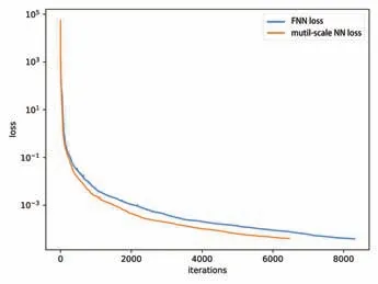
Fig 5 Comparison of convergence speed of loss function between FNN and multi-scale NN
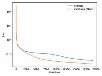
Fig 6 Comparison of convergence speed of loss function between FNN and multi-scale NN
In Table 3,we give the comparison of the relative L2error at different times when the FNN and the multi-scale NN are selected as the approximator in time iteration scheme(TIS).We can see that when using the multi-scale NN,the accuracy of the solution is higher and is improved by 64.7%at the final moment T=2.In Table 4,we perform sensitivity analysis on the number of boundary points and initial points,and give the relative L2error at the last moment T=2.We see that the accuracy of the solution is not significantly improved with the increase in the number of points.So we can select an appropriately small number of points to reduce the amount of calculation and achieve the required accuracy.

Table 3 Comparison of relative L2 error at different times for solving equations with two network structures

Table 4 Sensitivity analysis of the number of interior points and boundary points
3.3 3D Burgers Equation
we consider the following three-dimensional Burgers equation

where φ(x,y,z,t)=1+x+e-tsin(x)sin(y)sin(z), ∈=0.05.In this example, we set the structure of the multi-scale NN with 2 hidden layers, each layers with 100 neurons.At the same time, we choose tanh as the activation function, and set the time step to Δt=0.005,q=2.The m-scaling factor of the multi-scale NN is M=m×(1,1,2,2,···,i,i,···,25,25),where the hyperparameter m=0.06.The training set consists of N0=5×5×5 initial moment data pairs and Nb=21×21×6 boundary data pairs.In Fig 6,we give a comparison of the convergence speed of the loss function when TIS selects the FNN and the multi-scale NN as the approximator respectively.When we use a multi-scale NN,its loss function has a faster convergence rate as a whole.In Table 5,we give a comparison of the relative L2error at different times when TIS selects the FNN and the multi-scale NN as the approximator respectively.We see that when using a multi-scale NN,its solution accuracy is higher,and the accuracy of u,v,w at the final moment T=0.1 is increased by 45.3%,51.3%,61.5%,respectively.

Table 5 Comparison of relative L2 error at different times with two network structures
4 Conclusion
With the wide application of deep learning in many fields, our research on solving partial differential equations with deep learning becomes more important.We combine the neural networks with the traditional Runge-Kutta method, and establish a time iteration scheme approximation algorithm based on the multi-scale NNs,which alleviates the degradation of the accuracy of the numerical solution with time iteration to a certain extent.The introduction of the multi-scale NNs ensures that the convergence speed of the loss function is accelerated,and the accuracy of the numerical solution is also improved.In this way,we organically combine classical mathematical methods with NNs to provide new ideas for the numerical solution of partial differential equations.Since the time iteration scheme requires setting time-dependent input,sharing the parameters of the neural networks among multiple time step solutions.In future work,we continue to consider long short term memory networks and convolutional neural networks.

