Gang Zhang(張剛) Yu-Jie Zeng(曾玉潔) and Zhong-Jun Jiang(蔣忠均)

1School of Communication and Information Engineering,Chongqing University of Posts and Telecommunications(CQUPT),Chongqing 400065,China

2Cyberspace Administration of Guizhou Province,Guiyang 550000,China

Keywords: bearing fault detection,weak signal detection,piecewise linear symmetric tri-stable system,output signal-noise-ratio,adaptive genetic algorithm

1. Introduction

With the rapid development of mechanical fault detection technology,weak signal detection has become an important means of extracting fault characteristic signals,[1,2]but in many practical applications, fault signals are completely submerged in strong background noise. The low signal-tonoise ratio (SNR) makes traditional fault detection methods ineffective. Therefore,the effective extraction of fault signals in strong background noise is of great significance for practical engineering applications.[3,4]Traditional signal detection methods include wavelet decomposition,[5]ensemble empirical mode decomposition,[6]singular value decomposition,[7]etc. These methods are used mainly to detect signals by removing or suppressing noise, but the signals themselves are also suppressed to a certain extent at the same time. In view of this, the stochastic resonance(SR) first proposed by Benziet al.,[8]in 1981 can convert noise energy into signal energy without damaging the signal. Therefore,the SR has become a typical noise-enhancing signal method,which has been widely used in weak signal detection so far.[9]

In recent years, many scholars have conducted extensive researches of the classical bistable stochastic resonance system(CBSR)and achieved remarkable results,but the CBSR is only suitable for small parameters that satisfy the adiabatic approximation conditions.[10]In practical applications, the adiabatic approximation conditions cannot be satisfied because most of signals are large parameters and submerged in strong background noise. In order to achieve the better detection results and solve the practical problems in engineering applications, many scholars have conducted in-depth researches of SR systems. Lenget al.[11]proposed a second-sampling SR method, which compresses the collected signal and realizes SR through a nonlinear system. Wanget al.[12]proposed a detection method to reduce the correlation among system parameters through a special construction. The tri-stable model proposed by Zhanget al.[13]and Wanget al.[14]is applicable to the case of high noise in weak signal detection, and can better detect the early faults of rotating machinery under strong background noise conditions. Qiaoet al.[15]proposed an improved fractional-order SR model that can not only suppress the multiscale noise embedded in the signal,but also better characterize performance. An unsaturated piecewise system that solves the problem of system output saturation was proposed.[16–18]An SR system was applied to the bearing fault detection,and it was found that system parameters have great influence on system performance.[19–22]Hanet al.[23]derived the escape rate for particles by means of first passage time(MFPT).The system parameters are optimized by genetic algorithm in Refs.[24,25].

Moreover, most of the noise detected by weak signals is ideal Gaussian white noise, which cannot represent the random noise generated by non-anthropogenic activities in nature,[26]and its waveform has significant impulsive and trailing characteristics. In order to accurately simulate noise in various fields, stochastic resonance induced by Levy noise has attracted the attention of scholars in recent years. Jiaoet al.[27]studied the stochastic resonance phenomenon of asymmetric monostable systems under different Levy stable noise environments. Guet al.[28]systematically analyzed the mean first-passage time of asymmetric bistable system under Levy noise.

Although some research progress of weak signal detection as mentioned above has been made,further analysis shows that these systems only achieve single performance improvement by increasing the number of steady states or changing the structure of the potential function. Therefore, in order to solve the problem of output saturation and improve the output SNR of the system,a piecewise linear symmetric tri-stable random resonant system is proposed in this work. Firstly,under the premise of the adiabatic approximation theory, the SNR is deduced, and the influence of each parameter of the system on the SNR is analyzed,which is helpful in achieving the optimal detection effect. Then,in order to verify the practicality of the project,numerical simulation is introduced,and the simulation result is compared with that from the classical tristable stochastic resonance system(CTSR).In order to optimize the system parameters, an adaptive genetic algorithm is used to optimize the system parameters globally. Finally,the PLSTSR is applied to the bearing fault detection in Gaussian white noise and Levy noise,and the detection results are compared with the CTSR.

The rest of this paper is organized as follows. In Section 2 the CTSR and the PLSTSR proposed in this paper are described, and their saturation characteristics are discussed.In Section 3,the Kramers escape rate,MFPT and SNR of the PLSTSR are deduced and the effects of parameters on them are analyzed. Also the unsaturation of PLSTSR is proven and the adaptive genetic algorithm is introduced. In Section 4,the ability of PLSTSR to detect low-frequency, high-frequency,and multi-frequency signals in Gaussian white noise environment are verified. In Section 5, the practicability of the PLSTSR detection technology is verified through two bearing experiments under Gaussian white noise. In Section 6 the bearing fault detection capability of PLSTSR under Levy noise is proved, and its engineering application value is verified.In Section 7 some conclusions are drawn from the present research.

2. PLSTSR model

The dynamic equation of the classic stochastic resonance system is shown below.

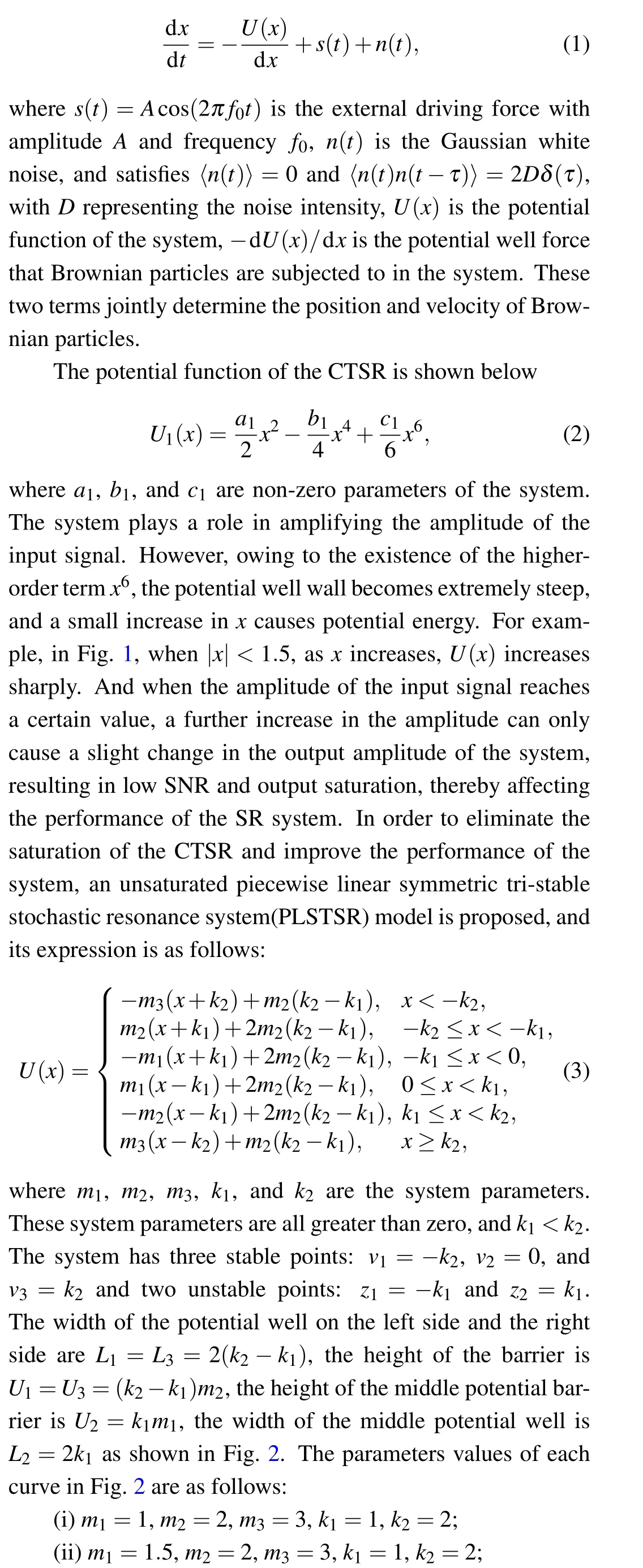
Fig.1. Potential function of CTSR.

It can be seen from Fig. 2, the system parameters exert large influences on the shape of the potential function. The changing ofm1,k1, andm2affect the change inU2,L2,U1respectively. Since the potential function of the PLSTSR is composed of 6 straight lines,the steepness of the barrier wall can be adjusted arbitrarily according to the system parameters.AsU(x)increases,xalso increases linearly,so the system does not saturate.

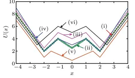
Fig.2. Potential function of PLSTSR.

A cosine signals(t)=0.2cos(2π×0.01t) is simulated under no noise, and the output signal waveform of the CTSR and the PLSTSR are shown in Fig.3 and Fig.4 respectively.

It can be seen from Fig. 3 that when the value ofAincreases from 0.2 to 0.4,the amplitude of the output signal increases significantly, and whenA>0.4, with the increase ofA,the amplitude of the output signal does not increase significantly, and it is maintained at around 1.5, the system is saturated. Figure 4 shows that as the input signal amplitude increases, the output signal amplitude increases proportionally,thus avoiding output saturation. Comparing Fig.3 with Fig.4,under the same input signal amplitude, the output signal amplitude of Fig.4 is much larger than that of Fig.3,indicating that the PLSTSR has better signal amplification capabilities than the CTSR.

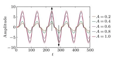
Fig.4. Output signal of PLSTSR.

3. SNR of PLSTSR

The output SNR is the method that is most commonly used to evaluate the performance of stochastic resonance system. Kramers escape rate and adiabatic approximation theory are used to derive the SNR of PLSTSR.Thep1(t),p2(t),andp3(t) are the residence probabilities of Brownian particles at the three stable points at timet. Ther12(t),r21(t),r23(t),andr32(t)are Kramers escape rates between stable points,respectively.TheT12,T21,T23,andT32represent the MFPTs of particles between two stable points respectively.[23]TheR12(t),R21(t),R23(t), andR32(t) are the probabilities of the particle transition between stable points at timet, respectively. According to Refs.[29,30],Taylor series expansion is performed on them under the condition of adiabatic approximation and the first term is taken as shown in Eqs.(6)and(7).

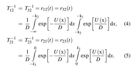
The MFPT can describe the difficulty of particle transition between potential wells,which can affect the occurrence of SR.Equation(6)shows thatT12andT32are only related tom2,m3,k1,andk2;T21,andT23are only related tom1andk1,;the curves of MFPT under parametersm1,m2,m3,k1,andk2are shown in Figs.5 and 6

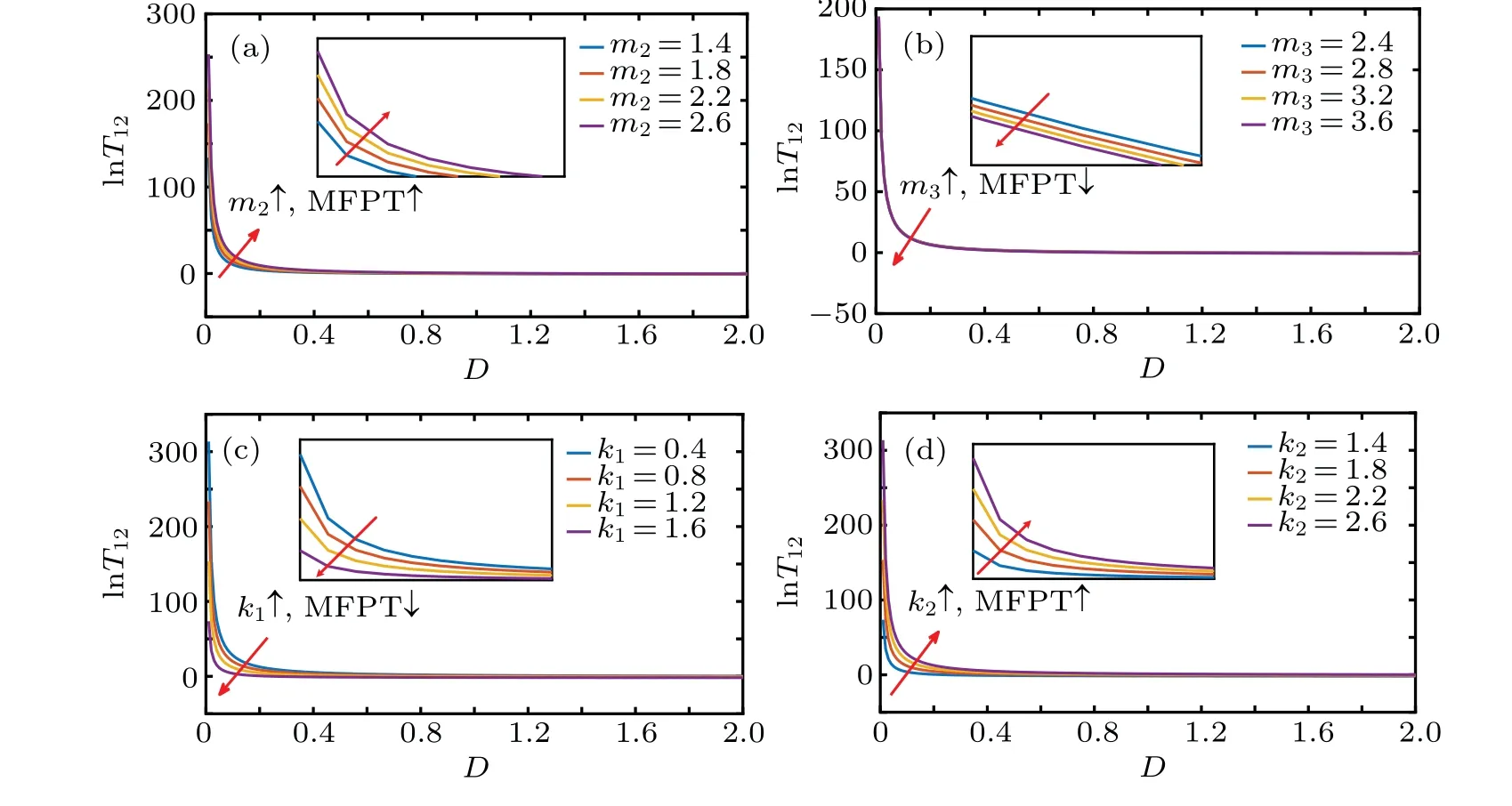
Fig.5. Variations of MFPT(v1 →v2)with D: (a)lnT12 changes with m2,(b)lnT12 changes with m3,(c)lnT12 changes with k1,(d)lnT12 changes with k2.

Fig.6. Variations of MFPT(v2 →v1)with D: (a)lnT21 changes with m1,(b)lnT21 changes with k1.

It can be seen from Figs. 5 and 6 that with the increase of noise intensity,the MFPT first gradually decreases and then tends to be stable,which indicates that the noise intensity can promote the transition of particles between potential wells,thereby generating stochastic resonance. Figure 5 show that MFPT(v1→v2)increases with the increase ofm2andk2and decreases with the increase ofm3andk1,indicating that the appropriate reduction ofm2andk2or appropriate increase ofm3andk1can promote the potential of particles from both sides.In Fig.6 that with the increase ofm1andk1,MFPT(v1→v2)increases, indicating that the appropriate reduction ofm2andk2can promote the transition of particles from the middle potential well to the potential wells on both sides.[30]

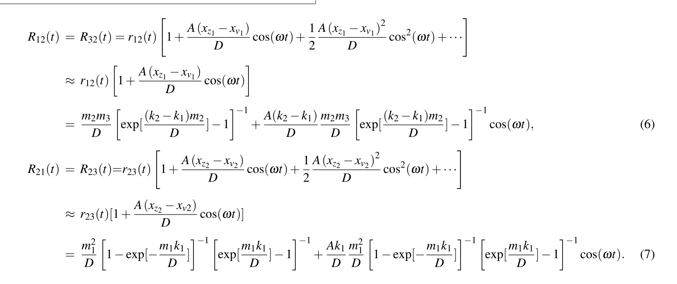
Equations(6)and(7)can be expressed by Eq.(8)and Eq.(9)respectively.

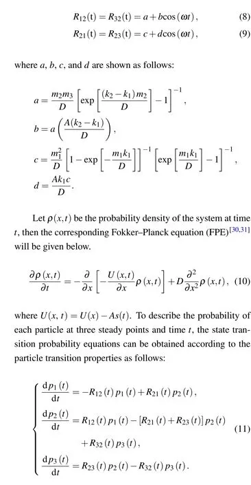
Substituting Eqs.(10)and(11)into Eq.(9),the linear ordinary differential method is used to solve the three-way homogeneous differential equation as given below

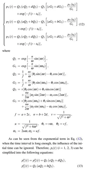
From Eq.(12),using the conditional probability theorem,the conditional probability shown in Eq.(14)can be obtained below.

According to the properties of transition probability in a symmetric system,equation(16)can be obtained as

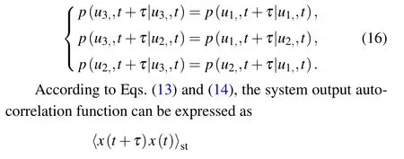
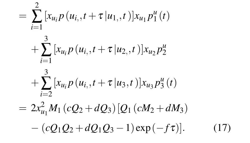
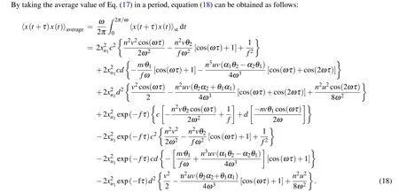
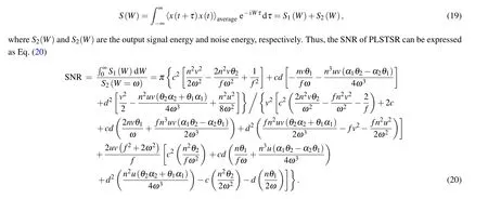
The output power of the signal can be obtained by the Fourier transform of autocorrelation function Eq.(18)below

3.1. Parameter selection

According to Eq.(20),the parameters can exert great influence on the value of SNR and determine the performance of the system. So it is necessary to study the influence of system parameters on the system. Lets(t)=0.2cos(2π×0.01t),then the relationship between SNR,noise intensity and system parameters will be shown in Figs.7–12.

In Fig.7,the PLSTSR has the characteristics of the classical stochastic resonance system. Given other parameters are fixed,with the increase of the noise intensity,the SNR shows a trend first increasing and then decreasing,where the appearing of the peak indicates that the stochastic resonance has occurred.

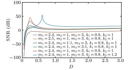
Fig.7. The change of SNR in PLSTSR with D.

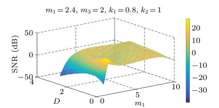
Fig.8. SNR versus D and m1.

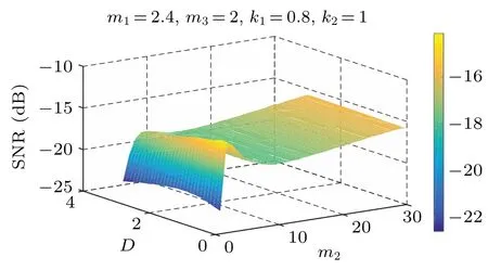
Fig.9. SNR versus D and m2.

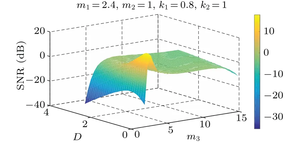
Fig.10. SNR versus D and m3.

It can be seen from Figs. 8–10, and 12 that withDand some parameters fixed,the SNR of the PLSTSR first increases and then decreases with any of the parametersm1,m2,m3,k2increasing, and its peak value also increases as parameterDincreases. Figure 11 shows that the SNR first increases and then decreases with the increase of parameterk1,which means that there is a traditional SR phenomenon. Unlike the changes of other parameters, the SNR increases with parameterk1increasing, but the position and size of the peak do not change as shown in Fig.9.

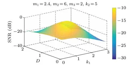
Fig.11. SNR versus D and k1.

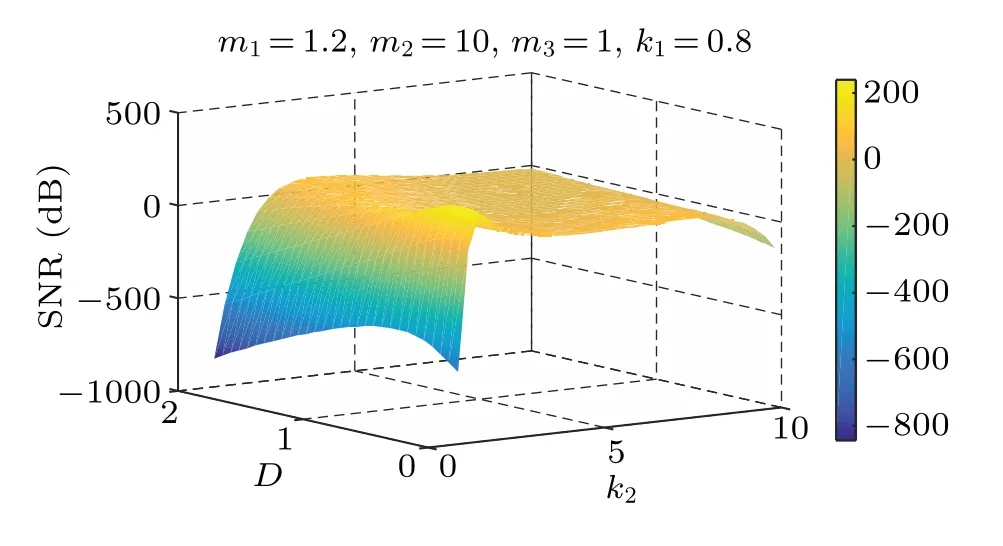
Fig.12. SNR versus D and k2.

3.2. Adaptive genetic algorithm(GA)

The above conclusions are all analyzed and discussed with part of the parameters fixed, but the coordinates of system parameters can also affect the performance of the system.Therefore, it is necessary to optimize these parameters. For example,many optimization algorithms such as adaptive iterative algorithm are only suitable for optimizing a small number of parameters. If there are too many parameters, then problems of insufficient precision and too high a computational complexity appear. However,the PLSTSR has 5 parameters,which is not suitable for the adaptive iterative algorithm.The adaptive genetic algorithm that simulates the biological genetic process has the advantages of multi-parameter optimization and high parameter accuracy.[24,25]Therefore,in this work the adaptive genetic algorithm is adopted to optimize the parameters. The SNR is used as the fitness function and the crossover operators such as those described Eq.(21)are used to construct the exclusive operator inX′=X+?.

The flowchart of GA is shown in Fig.11. Subsequent parameter optimization is based on a population size of 400, a genetic generation of 200, and a crossover probability of 0.4.The mutation probability of the PLSTSR is 0.1 and the mutation probability of the CTSR is 0.4.

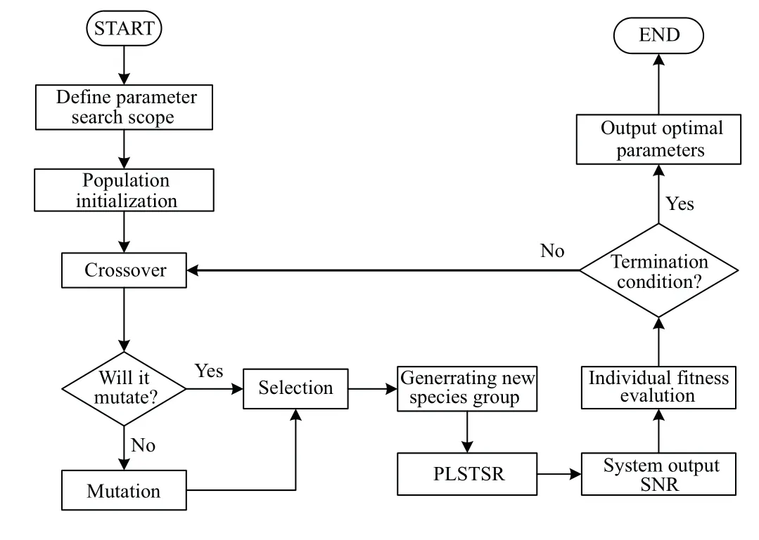
Fig.13. Flowchart of adaptive genetic algorithm.

4. Numerical simulation

4.1. Comparative analysis

In order to further prove the performance of PLSTSR,the fourth-order Runge–Kutta algorithm is used to simulate the periodic signals(t) = 0.2cos(2π×0.01t) in the Gaussian white noise environment, and the SNR is used as a measure.[32]Its definition is shown as follows:

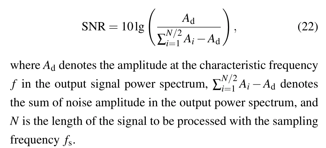
The optimal parameters of the PLSTSR are obtained by using the adaptive genetic algorithm:m1=2,m2=3,m3=3.5,k1=1,andk2=2. The optimal parameters of the CTSR area1=1,b1=2,andc1=0.1. After the 10th degree polynomial fitting,the SNR curve is obtained as shown in Fig.14.In Fig.14,with the increase ofD,the SNR for each of the two systems shows a trend first increasing and then decreasing,indicating a typical stochastic resonance phenomenon, but the peak value of the PLSTSR is larger,no matter whether the ambient noise is strong or weak,the value of SNR is larger than that of the CTSR,which proves the superiority of the PLSTSR.

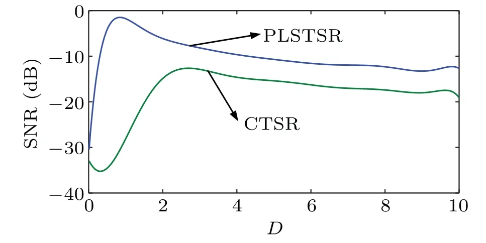
Fig.14. Comparison of SNR between PLSTSR and CTSR.

4.2. Weak signal detection

In order to further verify the performance of PLSTSR in signal detection,single-frequency signals(low-frequency signal and high-frequency signal)and multi-frequency signals are input into PLSTSR respectively, and the time-domain waveform and spectrum of the output signal are observed and compared with those in the case of CTSR.

4.2.1. Single-frequency signal detection

4.2.1.1. Low-frequency signal detection

The low-frequency signals(t)=0.2cos(2π×0.01t)and the Gaussian white noise ofD= 0.8 are used. The optimal parameters of the CTSR are given below:a1=0.4819,b1= 1.0028, andc1= 0.4003. The optimal parameters of the PLSTSR arem1= 0.0085,m2= 0.0489,m3= 0.1605,k1=0.2539,andk2=0.3316. Figures 15 and 16 are the time domains and spectrum waveforms of the input and output signals,respectively.

Fig.15. Time domain waveforms of input and output signals: (a)low-frequency cosine input signal,(b)low-frequency cosine input signal with noise,(c)CTSR output signal,(d)PLSTSR output signal.

Fig. 16. Powers spectrum of input signal and output signals: (a) low-frequency cosine input signal, (b) low-frequency cosine input signal with noise, (c)CTSR output signal,(d)PLSTSR output signal.

4.2.1.2. High-frequency signal detection

The high-frequency signals(t)=0.2cos(2π×11.5t) and the Gaussian white noise ofD=0.8 are used. The optimal parameters of CTSR area1=1.3007,b1=0.5162, andc1=0.0418. The optimal parameters of PLSTSR arem1=0.0651,m2=0.6589,m3=0.4605,k1=0.2653,andk2=0.4816. Figures 17 and 18 are the time domains and spectrum waveforms of the input and output signals,respectively.

Fig.17. Time domain waveforms of input and output signals. (a)High-frequency cosine input signal,(b)high-frequency cosine input signal with noise,(c)CTSR output signal,(d)PLSTSR output signal.

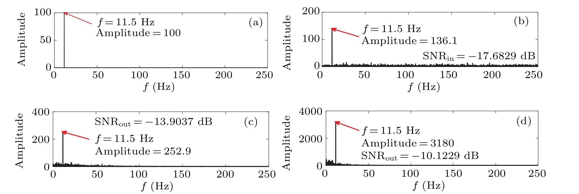
Fig.18.Power spectra of input signal and output signals:(a)high-frequency cosine input signal,(b)high-frequency cosine input signal with noise,(c)CTSR output signal,(d)PLSTSR output signal.

4.2.2. Multi-frequency signal detection

The multi-frequency signals(t)=0.1cos(2π×0.01t)+0.2cos(2π×0.03t)+0.3cos(2π×0.05t)and the Gaussian white noise ofD=0.8 are used. The optimal parameters of CTSR area1=0.2819,b1=0.7632, andc1=0.5118. The optimal parameters of PLSTSR arem1=0.0158,m2=0.0169,m3=0.3558,k1=0.2169,andk2=0.4308. Figures 19 and 20 are the time domains and spectrum waveforms of the input and output signals,respectively.

Fig.19. Time domain waveforms of input and output signals: (a)multi-frequency input signal,(b)multi-frequency input signal with noise,(c)CTSR output signal,(d)PLSTSR output signal.

Fig. 20. Power spectra of input signal and output signals: (a) multi-frequency input signal, (b) multi-frequency input signal with noise, (c) CTSR output signal,(d)PLSTSR output signal.

4.2.3. Summary

As can be seen from Figs.15–20,the PLSTSR can detect low-frequency,high-frequency,and multi-frequency signals well,indicating wide range of applications. Compared with the CTSR,the PLSTSR has very high output signal amplitude and signalto-noise ratio as shown in Tables 1 and 2.

Table 1. Comparison of performance between different systems in weak signal detection.

Table 2. Comparison of SNR between different systems in weak signal detection.

5. Bearing fault detection under Gaussian white noise

5.1. Bearing the fault detection for 6205-2RS JEM SKF model

To prove the great potential of the PLSTSR proposed in this paper in practical engineering applications,the CTSR and PLSTSR are used to detect the bearing fault data of Case Western Reserve University(CWRU).The bearing model is 6205-2RS JEM SKF, and the experimental workbench is shown in Fig. 21. The main parameters are shown in Table 3.[33,34]Since the adiabatic approximation theory needs to satisfy the condition of small parameters,the stochastic resonance is generated by the method of second-sampling. The sampling frequency isfs=12000 Hz, the number of sampling points isN=10000, and the secondary sampling frequency isfsr=5 Hz. In order to improve the fault detection performance of the system,an adaptive genetic algorithm is used to obtain the optimal parameters. By comparing the consistency between the characteristic frequency and the detection frequency,it can be judged whether a fault occurs. The calculation of the characteristic frequency is shown in Eq.(23).

wherefr=29.9 Hz is the rotational frequency of the bearing. By substituting the data in Table 3 into Eq. (23), the fault frequencies of the inner and outer rings of the bearing can be calculated to befBPFI=162.2 Hz andfBPFO=107.3 Hz,respectively. Secondly, the sampling frequency is set to befs=12000 Hz, the sampling pointN=10000 and the secondary sampling frequencyfsr=5 Hz to preprocess the fault signal so as to meet the adiabatic approximation condition.

Fig.21. 6205-2RS JEM SKF deep groove ball bearing test device.

5.1.1. Inner ring fault detection

Figures 22(a)and 23(a)show the time–frequency diagram of the 6205-2RS JEM SKF inner ring bearing fault signal. Figures 22(b)and 23(b)are time–frequency diagrams of the fault signal after adding Gaussian white noise. Figures 22(c)and 22(d)and figures 23(c)and 23(d)show the time–frequency diagrams of the output signals of the CTSR and PLSTSR respectively. The optimal parameters of the CTSR area1=2.4876,b1=1.1249, andc1=0.003. The optimal parameters of the PLSTSR arem1=0.4312,m2=1.4347,m3=1.0996,k1=0.0342,andk2=0.0838.

Fig. 22. Time domain waveforms of input and output signals: (a) inner ring fault input signal, (b) inner ring fault signal with noise (D=0.2), (c) CTSR output signal,(d)PLSTSR output signal.

Fig.23. Power spectra of input signal and output signals: (a)inner ring fault input signal,(b)inner ring fault signal with noise,(c)CTSR output signal,(d)PLSTSR output signal.

It can be seen from Figs. 22(c) and 22(d) that the amplitude of the time domain waveform of the output signal of PLSTSR is significantly larger than that of the CTSR,and the periodicity is stronger. Figures 23(c)and 23(d)show the peak of PLSTSR and CTSR atf=162 Hz(relative error is 0.12%),which are 8.748 and 32.21 respectively, so the PLSTSR is 23.462 higher than that of CTSR. The SNRs of the two systems are?13.0787 dB and?10.8274 dB respectively,and the PLSTSR is 2.2513 dB higher than the CTSR,which proves the advantage of the PLSTSR in fault signal detection.

5.1.2. Outer ring fault detection

Figures 24(a) and 25(a) show the time–frequency diagram of the 6205-2RS JEM SKF outer ring bearing fault signal. Figures 24(b) and 25(b) show the time–frequency diagrams of the fault signal after adding Gaussian white noise.Figures 24(c) and 24(d) and Figs. 25(c) and 25(d) show the time–frequency diagram of the output signals of the CTSR and PLSTSR respectively. The optimal parameters of the CTSR area1=0.1507,b1=0.5291,andc1=0.3201. The optimal parameters of the PLSTSR arem1= 1.9598,m2= 1.3831,m3=5.6892,k1=3.5269,andk2=4.0129.

It can be seen from Fig. 24 that the time domain waveform of the PLSTSR output signal has stronger periodicity and larger output amplitude. It can be seen from Figs. 25(c)and 25(d) that the spectral peaks of the output signals of the two systems are both atf= 108 Hz (relative error is 0.65%), but the spectral peak of the CTSR output signal is only 2.419,while the spectral peak of the PLSTSR output signal is 1269.The SNR of PLSTSR and CTSR are?14.2030 dB and?5.5644 dB,respectively,and the PLSTSR is 7.6389 dB higher than the CTSR.

Fig. 24. Time domain waveforms of input and output signals: (a) outer ring fault input signal, (b) outer ring fault signal with noise (D=0.8), (c) CTSR output signal,(d)PLSTSR output signal.

Fig.25. Power spectra of input signal and output signals: (a)outer ring fault input signal,(b)outer ring fault signal with noise(D=0.8),(c)CTSR output signal,(d)PLSTSR output signal.

5.2. Bearing fault detection under LDK UER204 model

Currently, the experimental data which are widely used by many scholars of SR are the CWRU bearing fault data public set. Therefore, in order to verify the applicability of the PLSTSR in different scenarios, the national public data LDK UER204-type bearing is selected for the experiment. The experimental device is shown in Fig.26. The bearing structural parameters[35]are shown in Table 4. The sampling frequency is set to befs=25600 Hz,sampling pointN=20000,and the theoretical value of outer ring fault frequency is calculated to bef=107.91 Hz. Since the signal does not meet the adiabatic approximation condition either, the secondary sampling frequency is set to befsr=5 Hz.

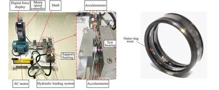
Fig.26. LDK UER204 bearing test device.

Table 4. Main data of LDK UER204 bearing.

5.2.1. Outer ring fault detection

Figures 27(a)and 28(a)show the time–frequency diagram of the LDK UER204 bearing fault signal. Figures 27(b) and 28(b) show the time–frequency diagrams of the fault signal after adding noise. Figure 27(c) and 27(d) and figures 28(c)and 28(d) show the time–frequency diagrams of the output signals of the CTSR and PLSTSR, respectively. The optimal parameters of the CTSR area1=0.1007,b1=2.6162,andc1=0.0418. The optimal parameters of the PLSTSR arem1=1.1512,m2=1.0547,m3=1.3156,k1=0.4354, andk2=0.5677.

Fig. 27. Time domain waveforms of input and output signals: (a) outer ring fault input signal, (b) outer ring fault signal with noise (D=0.2), (c) CTSR output signal,(d)PLSTSR output signal.

Fig. 28. Power spectra of input signal and output signals: (a) outer ring fault input signal, (b) CTSR output signal, (c) PLSR output signal, (d) PLSTSR output signal.

From Figs. 28(a) and 28(b), it can be seen that the fault frequency cannot be identified by directly using Fourier transform to obtain the power spectrum of the original fault signal nor the noise-added fault signal. In Figs.28(c)and 28(d),the spectral peaks of both systems are atf=107.5 Hz(relative error is 0.38%)with peaks of 0.3402 and 5.75 respectively. The SNR of the two systems are?23.1750 dB and?20.2316 dB,respectively. The PLSTSR is improved by 2.9434 dB relative to CTSR.Obviously,the PLSTSR has a larger peak and SNR,less noise interference which makes it easier to detect the fault signal.

6. Bearing fault detection under Levy noise

Since Gaussian white noise is an ideal noise and cannot effectively simulate the actual noise in engineering practice,non-Gaussian Levy noise is introduced in order to be more similar to the random noise in the actual engineering environment.

6.1. Levy noise

The characteristic function expression of Levy noise[36]is shown as follows:

where is the characteristic parameter,which determines the smearing characteristics and impulse characteristics of its distribution.The smearing characteristics of the noise turns stronger as increases,and the impulse characteristics becomes weaker as increases.The is a symmetry parameter, which determines the symmetry of the distribution. is the scale parameter, and represents the position parameter,which determines the center position of the distribution.

The random variables of Levy noise are generated by the Chambers–Mallows–Stuck(CMS)method.

where the random variablesVandWare independent of each other,V ∈(?π/2,π/2) obeys a uniform distribution,Wfollows an exponential distribution with a mean of 1, andCα,β= arctan(βtan(πα/2))/α,Dα,β,σ=σ[cos(arctan(βtan(πα/2)))]?1/α.

6.2. Bearing fault detection under LDK UER204 model

In order to verify the ability of PLSTSR to detect th bearing fault under Levy noise, the same LDK UER204 type of bearing as that in the previous section is selected. The sampling frequency is set to befs=25600 Hz, sampling pointN=20000, and the theoretical value of outer ring fault frequency is calculated to befout=107.91 Hz. Since the signal does not meet the adiabatic approximation condition either,the secondary sampling frequency is set to befsr=5 Hz.

Figures 29(a) and 30(a) show the time–frequency diagrams of the LDK UER204 bearing fault signal, and figures 29(b) and 30(b) display the time–frequency diagrams of the fault signal after adding Levy noise. None of the characteristic frequencies of the fault signals can be identified. Figures 29(c) and 29(d) and figures 30(c) and 30(d) show the time–frequency diagrams of the output signals of the CTSR and PLSTSR, respectively. The optimal parameters of the CTSR area1=0.7112,b1=1.562,andc1=0.2311.The optimal parameters of the PLSTSR arem1=4.4652,m2=5.0647,m3=9.0956,k1=1.3354,andk2=1.6697.

Fig.29. Time domain waveforms of input and output signals. (a)Outer ring fault input signal, (b)outer ring fault signal with noise(D=0.2), (c)CTSR output signal,(d)PLSTSR output signal.

Fig.30. Power spectra of input signal and output signals: (a)outer ring fault input signal,(b)outer ring fault signal with noise,(c)CTSR output signal,(d)PLSTSR output signal.

Comparing spectra among Figs. 30(a)–30(d), only the spectral peak of PLSTSR output signal is located atf=107.5 Hz (relative error is 0.38%), the CTSR cannot detect fault frequency well in Levy noise environment. Although the noise utilization rate of PLSTSR is not ideal, the fault frequency can still be detected. The SNR at fault frequency is?19.8919 dB,and the relative input SNR is also improved by 25.684 dB,which proves the engineering application value of PLSTSR.

7. Conclusions and perspectives

In this work,the PLSTSR is proposed and applied to the detecting of low-frequency, high-frequency, multi-frequency signal,and bearing fault under Gaussian white noise and Levy noise. The PLSTSR is introduced, its saturation is verified,and the Kramers escape rate and MFPT are derived. Then,using the SNR as a measure,the influence of system parameters on the SNR is analyzed.Some conclusions are drawn from the present research as follows.

(i)PLSTSR overcomes the saturation of CTSR,improves the system output SNR,and amplifies the signal amplitude.

(ii) The adaptive genetic algorithm optimizes the system parameters collaboratively,so that the results can achieve global optimization.

(iii) The PLSTSR can detect low-frequency, highfrequency and multi-frequency signals well, and its SNR and output amplitude are better than those of the CTSR.

(iv) The PLSTSR is applied to the bearing fault detection of two scenarios under the Gaussian white noise, which eliminates the chance that the proposed system is only suitable for a certain bearing. The experimental results show that the PLSTSR has better large output amplitude and SNR.It is proved that the system has good theoretical significance and practical value. The details are shown in Table 5.

(v) The PLSTSR and CTSR are applied to detecting of bearing fault under the Levy noise, which proves that the PLSTSR can also detect fault signals in a noise environment closer to engineering scenario,while the CTSR cannot detect fault signals. The specific test results are listed in Table 5.

Table 5. Comparison of performances among different systems in bearing fault detection.

The system proposed in this paper is a one-dimensional system. Subsequent research will apply the potential function of PLSTSR to a two-dimensional system or an underdamped system,and judge its superiority in performance.

Acknowledgements

Project supported by the National Natural Science Foundation of China (Grant No. 61771085), the Research Project of Chongqing Educational Commission,China(Grant Nos. KJ1600407 and KJQN201900601), and the Natural Science Foundation of Chongqing, China (Grant No.cstc2021jcyj-msxmX0836).