Laser-induced breakdown spectroscopy for the classification of wood materials using machine learning methods combined with feature selection
Xutai CUI (崔旭泰), Qianqian WANG (王茜蒨), Kai WEI (魏凱),Geer TENG (騰格爾) and Xiangjun XU (徐向君)
1 School of Optics and Photonics, Beijing Institute of Technology, Beijing 100081, People’s Republic of China
2 Key Laboratory of Photonic Information Technology, Ministry of Industry and Information Technology,Beijing 100081, People’s Republic of China
Abstract In this paper,we explore whether a feature selection method can improve model performance by using some classical machine learning models, artificial neural network, k-nearest neighbor,partial least squares-discrimination analysis,random forest,and support vector machine(SVM),combined with the feature selection methods, distance correlation coefficient (DCC), important weight of linear discriminant analysis(IW-LDA),and Relief-F algorithms,to discriminate eight species of wood (African rosewood, Brazilian bubinga, elm, larch, Myanmar padauk,Pterocarpus erinaceus, poplar, and sycamore) based on the laser-induced breakdown spectroscopy (LIBS) technique.The spectral data are normalized by the maximum of line intensity and principal component analysis is applied to the exploratory data analysis.The feature spectral lines are selected out based on the important weight assessed by DCC,IW-LDA,and Relief-F.All models are built by using the different number of feature lines(sorted by their important weight)as input.The relationship between the number of feature lines and the correct classification rate (CCR) of the model is analyzed.The CCRs of all models are improved by using a suitable feature selection.The highest CCR achieves (98.55...0.39)% when the SVM model is established from 86 feature lines selected by the IW-LDA method.The result demonstrates that a suitable feature selection method can improve model recognition ability and reduce modeling time in the application of wood materials classification using LIBS.
Keywords: laser-induced breakdown spectroscopy (LIBS), feature selection, wood materials
1.Introduction
Wood is an important biological material that consists of complex components and includes a wide variety of existing species[1].The physical and chemical properties of different wood species are distinct and influence their application.In the field of biodiversity, environmental conservation, and industry,etc,the recognition of wood species is a crucial step[2–4].However, the classification of different wood species based on manual visual methods has a high cost and lacks automaticity and high efficiency [5].Therefore, it is essential to develop an automatic technology that can classify the species of wood materials efficiently and accurately for research and application of wood materials.
Several analytical techniques have been reported to discriminate the species of wood materials, for example, mass spectrometry [6, 7], the chemiresistor gas sensor array [8],thermogravimetric analysis [9], molecular fluorescence [10],near-infrared spectroscopy [11–13], Raman spectroscopy[14],and x-ray fluorescence spectroscopy[15,16].However,these techniques require some sample preparation, which increases the complexity of the measurement.Besides, these techniques mentioned above might require a laboratory environment,which could not be used forin situapplications[17, 18].Laser-induced breakdown spectroscopy (LIBS) as a powerful elemental analysis technique has some unique advantages such as rapid analysis, little or no sample preparation, operationin situ, and remote measurement [19–21].Thus,the classification of wood species using LIBS combined with chemometric methods has been proposed[22,23].In the analytical process of LIBS,the sample surface is ablated by a laser pulse with high energy and a laser-induced plasma is generated.Then,the plasma decays and emits radiation which contains the element-specific information.The emission is detected and collected by a spectrometer and transformed into spectral data, which are transferred to the computer.The element-specific information of the sample is obtained by using the corresponding spectral analysis methods.
LIBS combined with a machine learning model has already been reported [24, 25].These research reports are mainly focused on the model and the corresponding parameter optimization process.However, besides the factors mentioned above that could influence the model performance,another factor influencing the performance of the classification model is input data.Selecting suitable feature variables as input data can avoid over-fitting and improve the correct classification rate (CCR) because the feature variables will contribute more in identification and feature selection can avoid interference from noise and irrelevant signals.In our previous work [23], LIBS combined with the artificial neural network (ANN) was investigated to classify four species of wood samples.The loadings of principal component analysis(PCA) are regarded as the criterion to select the input variables but the optimization process and discussion were mainly focused on the parameter setting of the ANN model.The influence of feature selection on the performance of classification models was not discussed in detail.To pick a suitable feature selection algorithm for a specific classification task,it is necessary to analyze the impact of feature selection on some classical machine learning models.
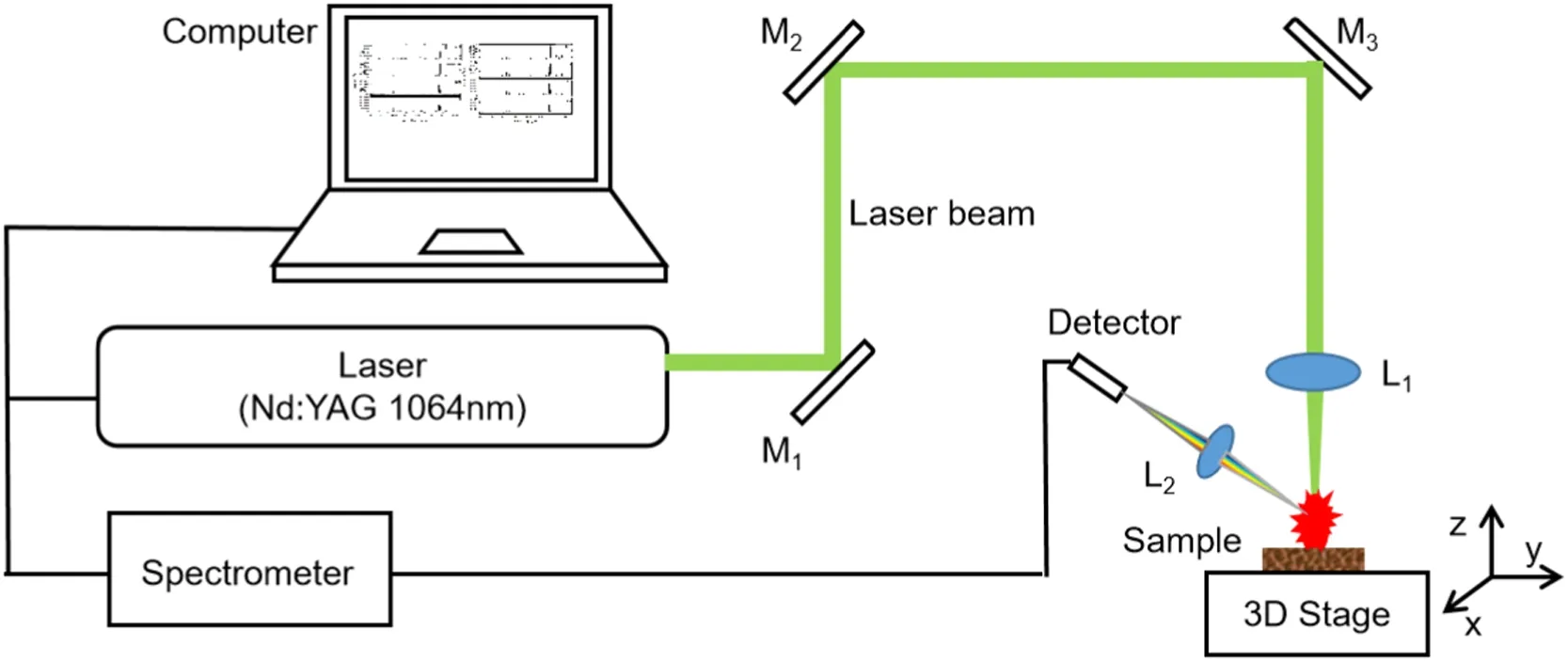
Figure 1.LIBS experimental setup for wood species analysis.
In general, LIBS data consist of many spectral variables due to the wide wavelength range and high spectral resolution[26, 27].However, a large number of the variables might be redundant information or noise.As machine learning or a chemometrics method has become a routine operation to analyze LIBS data, the redundant information or noise might reduce the recognition ability and computational performance of the corresponding methods [28].Therefore, some feature selection methods are performed before the quantitative or qualitative analysis of LIBS data.Some research work has proved that using selected feature variables can improve the model performance, for example, improving the calculation rate, reducing the amount of computation, and removing the interference, etc.There are some feature selection methods based on manual methods[29],random forest(RF)[30],PCA loadings [23], genetic algorithm (GA) [31], and partial least squares discriminant analysis (PLS-DA) [32].The manual methods are simple to handle but it depends on experience and the accuracy of this method is hard to ensure for the samples with a similar element composition.The RF model has great robustness for noise and can avoid the over-fitting phenomenon but the parameters optimization process is complicated [33].The PCA loadings method is easy to perform but the performance is unstable since the supervised information is not used.The GA has great performance but the optimization process needs iteration of evolution.The PLS-DA model needs to optimize the number of latent variables and is more suitable for a binary classification task.These methods mentioned above might increase the complexity in the process of data analysis so it is necessary to find some simple and effective feature selection methods to use in the multi-classification task.The distance correlation coefficient(DCC),linear discriminant analysis(LDA),and Relief-F algorithm, which are easy to perform and have high efficiency, might be able to achieve the feature selection task.Therefore,we employ DCC,LDA,and the Relief-F algorithm to select features in this research.
In this paper, eight different species of wood materials(African rosewood, Brazilian bubinga, elm, larch, Myanmar padauk,Pterocarpus erinaceus, poplar, and sycamore) are selected as the samples.LIBS spectral data of these wood samples are recognized by five classical chemometrics models,ANN,k-nearest neighbor(kNN),PLS-DA,RF,and SVM.Feature variables are selected out by DCC,IW-LDA,and the Relief-F algorithm.The relationship between the number of feature variables and the correct CCR of the model is analyzed.Meanwhile, the suitable feature selection method is chosen by comparing the training time and optimal CCRs of these models built based on feature variables evaluated by DCC, IW-LDA, and the Relief-F algorithm.
2.Materials and methods
2.1.Experimental setup
The experimental setup is the same as the LIBS system used in the previous work [23], which is shown in figure 1.A Q-switch flashlamp-pumped Nd:YAG laser operating at 1064 nm wavelength is used as the excitation source(~85 mJ pulse energy, 13 ns pulse duration, and 1 Hz repetition rate).
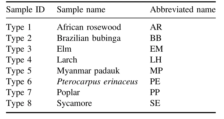
Table 1.The sample ID, sample name, and abbreviated name of wood species.
The laser beam is guided through three reflectors (M1, M2,and M3) and focused on the surface of wood samples by a convex lens(L1)with a 100 mm focal length.The diameter of the laser spot is about 600 μm and the laser fluence is 2.3 GW cm?2approximately.The wood samples are put on a threedimensional translation stage and moved by the translation device to ensure that each laser pulse can ablate a fresh location.The laser is preheated for half an hour before measurement to stabilize the laser energy.
Plasma emission generated by the ablated sample is focused and collected into a fiber optic bundle (two-fiber,each of 600 μm diameter)by a convex lens(L2)with a 36 mm focal length.The angle between the normal direction of L2and the incidence direction of the laser beam is about 45°.The fiber bundle connects with a two-channel gated charge-coupled device (CCD) spectrometer (AvaSpec 2048-2-USB2,Avantes).The spectral range covers from 200 nm to 950 nm with a convertible spectral resolution of 0.20–0.30 nm.The acquisition parameters of the spectrometer are set by software(AvaSpec 7.6 provided by Avantes).In this experiment, the delay time, which is the time interval between the flash lamp trigger and the spectrometer acquisition, is 376 μs and the integration time of the CCD is 2 ms.The experiment is conducted under ambient conditions.
2.2.Materials
The wood samples, which are already manufactured into 140 mm×80 mm×5 mm blocks, are purchased at a local market in China.The names of the woods(African rosewood,Brazilian bubinga,elm,larch,Myanmar padauk,Pterocarpus erinaceus, poplar, and sycamore) and the corresponding sample IDs are listed in table 1.For each type of wood sample,there are two blocks selected randomly,one is used to collect training spectra and the other is used to collect test spectra.All samples are cleaned with alcohol.The surface of the wood block is divided into 100 regions with the same size and each region(14 mm×8 mm)is regarded as one sample.In the experiment, three laser shots ablate at different positions in each region and these three spectra are averaged into one spectrum.For each type of wood, 100 training spectral data and 100 test spectral data are obtained.Finally,there are 800 training set data and 800 test set data in total.The training data are used for establishing classification models.The test data are used to assess the performance of the model.

Figure 2.(a)The description of the DCC method and(b) flow chart of feature selection method based on the DCC.
3.Feature selection algorithms

Figure 3.The averaged LIBS spectra of eight species of wood samples.
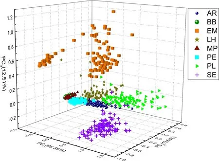
Figure 4.PCA score of spectral data in the training set (100 spectra for each species),which are explained by the first 3 PCs in 91.39%.
Data processing and analysis procedures include data preprocessing, feature variable selection, and classification.In this work,normalized by the maximum is selected as the data preprocessing, the methods based on DCC, IW-LDA, and Relief-F are used to select the feature variables,and five kinds of classical machine learning models (ANN,kNN, PLS-DA,RF, and SVM) are used to classify the spectra of wood samples.The improvement of model CCR is regarded as a criterion to evaluate the performance of the feature selection method.The algorithms of these classification models have been described in our previous work [34].The principles of DCC,IW-LDA,and Relief-F algorithms are described briefly.
3.1.Distance correlation coefficient (DCC)
The DCC is a correlation measurement method that can describe both the linear and nonlinear correlation between two variables.The value range of the DCC is within 0–1 and the correlation between the two variables is stronger if the value of the DCC is higher.When the DCC is zero,it can be claimed that the two variables are independent.The description of the DCC method and the flow chart of the feature selection method based on DCC are shown in figure 2.In the process of the feature selection method based on DCC, the spectral data are utilized to establish the spectral data matrix,which is anM-by-Pmatrix (MandPare the numbers of all spectral data and spectra lines, respectively).The label of class just means the category information rather than quantitative information.Hence,the‘one-hot encoding’method is used to create the label matrix, which is anM-by-N(Nis the number of classes) response matrix in which the rows and columns correspond to the response of observations and category information,respectively.The column of the spectral data matrix is U and the column of the ‘one-hot encoding’label matrix is V.For each spectral line,the DCCs between its corresponding column of the spectral data matrix and all columns of the‘one-hot encoding’label matrix are calculated.The important weight of this spectral line is the maximum among theseNvalues of DCCs.
3.2.Important weight of linear discriminant analysis (IW-LDA)
IW-LDA evaluates the importance of variables by calculating the projection matrix, W, of LDA.LDA is a classical linear learning algorithm, which can be generalized to multi-classification tasks [35].Suppose that the data set can be identified intoNclasses and the number of theith class ismi, the within-class scatter matrix, Sw, and between-class scatter matrix, Sb, can be obtained by equation (1),

where x, ui, u, and Xiare the data, averaged value of data in theith class, averaged value of all data and data set within-class, respectively.The projection matrix, W, is the matrix that consists of the eigenvectors corresponding to the firstd’ largest non-zero generalized eigenvalues ofSb,d′≤N?1.The proportions of the eigenvalues to the sum ofd’ largest non-zero generalized eigenvalues are regarded as the explanation, e.The variables are ranked by absolute values of e·W in descending order.
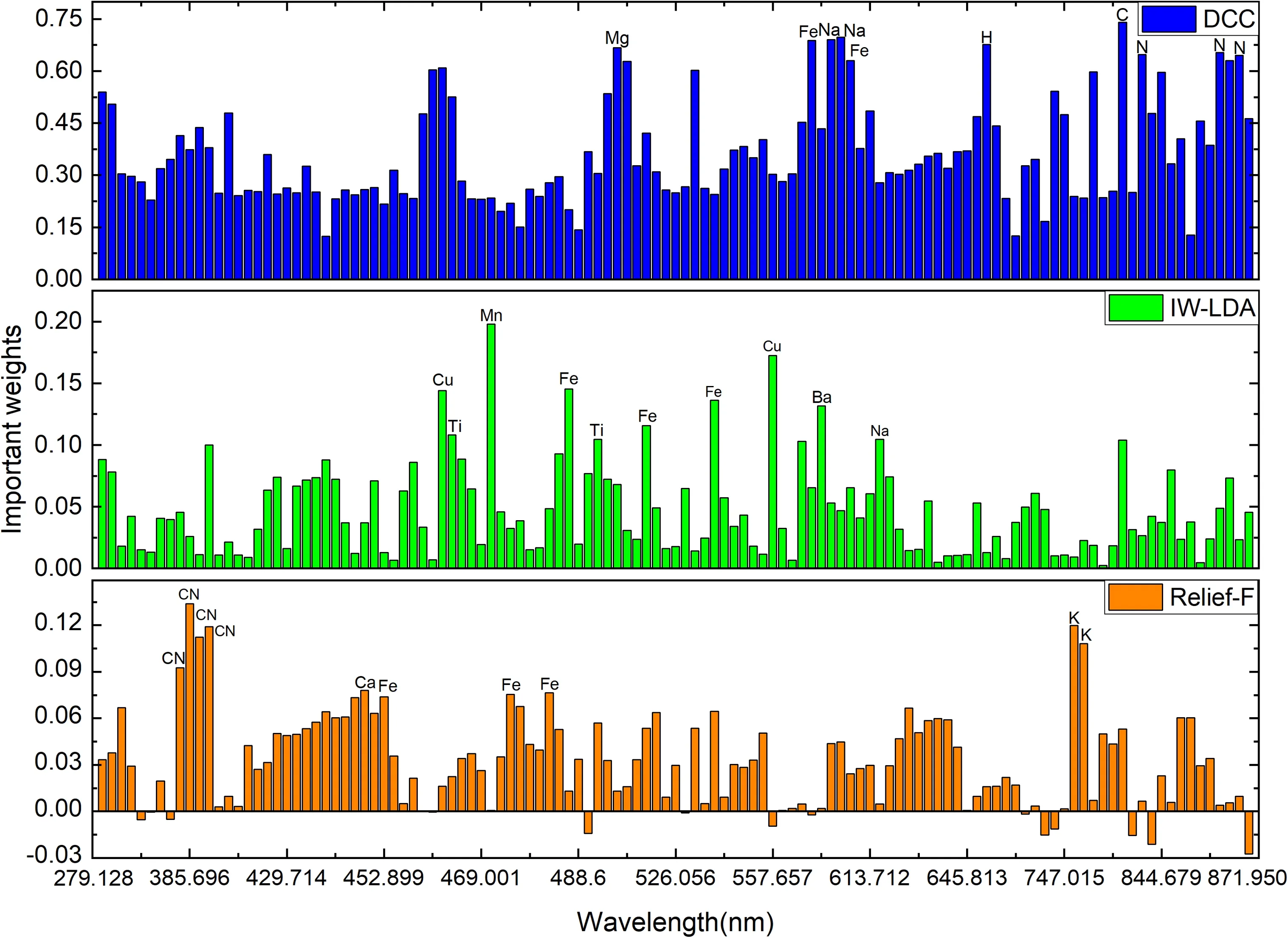
Figure 5.The important weights were evaluated by DCC, IW-LDA, and Relief-F.The top ten variables selected by each feature selection method are marked in the figure.
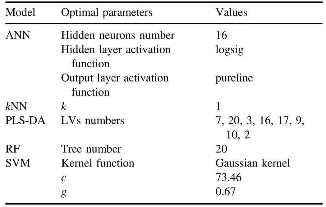
Table 2.The optimal parameters of all models.
3.3.Relief-F algorithm
Relief-F is an extended version of Relief that is a classical filtering feature selection method.The Relief method evaluates the importance of variables by correlation.Relief is just a method for the binary classification task while Relief-F can deal with the multi-classification.Hypothesize that the data setDconsists ofNclasses of data.If dataxibelongs to thekth class (k∈{1, 2,...,N}), firstly, Relief-F will select out the nearest dataxi,k,nhin thekth class and the nearest dataxi,l,nm(l=1, 2,...,N;l≠k) in other classes as near-hit and nearmiss, respectively.In our research, the metric used for determining the nearest data is the shortest Euclidean distance.Then,the correlation of thejth attribution is calculated by equation (2),

whereplis the proportion of thelth to the whole data set.
4.Results and discussion
4.1.LIBS spectra
The LIBS spectra of eight species of wood samples are shown in figure 3.Emission lines from Ca (422.41 nm, 445.11 nm),Fe (392.788 nm, 396.47 nm, 611.1 nm, and 615.2 nm),H(656.1 nm),N(742.364 nm,744.306 nm,and 766.523 nm),Na (588.95 nm and 589.55 nm), O (777.21 nm), and CN molecular violet bands (383–389 nm) can be observed in the spectra of all eight species of wood samples.However, some intensities of these spectral peaks are different for the eight wood species.For example,the intensity of O(777.21 nm)inthe spectrum of AR and the intensity of Fe (392.788 nm) in the spectrum of BB are weaker compared to the other wood species.The ratio of O to Fe(O/Fe)in the spectrum of MP is 1.73 and the value of O/Fe in PE is 0.90,approximately.It is worth noting that the intensities of such spectral data and the ratio between them are the key factors in distinguishing the wood species.The initial spectra data are composed of 3466 variables, including background, noise, and elemental information.All the obvious 119 lines intensities (the area of the single emission line) of the elements and molecules (including C, CN, C2,H, N,O, Ca,Cr, Ba,Fe,K, Mg,and Na,etc)are calculated in the whole wavelength range (200–900 nm)as input variables for data processing and analysis.

Table 3.The CCRs, training time, and prediction time of all models.
4.2.Principal component analysis (PCA)
Before the normal classification, exploratory data analysis(EDA) is performed to analyze and visualize data initially.PCA is one kind of the most commonly EDA methods used for preliminary data analysis to provide an overview of the data distribution.Therefore, PCA is used first for analyzing the spectral data of wood species.Figure 4 shows the PCA result of the training data(100 spectra for each species,800 in total) in the first three PCs.Each species is shown with different colors and shapes for better visualization.
The first three PCs accumulate 91.39% of the total variance.The spectra of EM, SE, LH, and PL species show a clear distinction compared with the rest of the wood samples.In contrast, spectra belonging to BB and MP species are overlapping with each other but distinct from other spectra,while the spectra of AR and PE species are mixed because the scores of spectra from AR and PE species factors are very close in the first three PCs,which means the spectra from AR and PE species are hard to classify just using the first three PCs.The PCA results show that spectra of EM, SE, LH, and PL species might be easy to recognize.However, PCA does not provide any classification results.Thus, the classification models are necessary to classify the spectra of eight species of wood.
4.3.Feature variables selection
The feature selection methods based on the DCC, IW-LDA,and Relief-F are performed on the training set.The importance of all variables (119 in total) evaluated by DCC, IWLDA,and Relief-F is obtained.Figure 5 shows the important weights of all variables evaluated by DCC, IW-LDA, and Relief-F.The top ten variables selected by each feature selection method are listed in figure 5.
Figure 5 shows that the important weights evaluated by DCC, IW-LDA, and Relief-F are different.For DCC results,the top ten variables,including C,Fe,H,N,Na,and Mg lines,are distributed in the range 500–900 nm.For IW-LDA results,the top ten variables (Ba, Cu, Fe, Mn, Na, and Ti) are distributed in the range 400–500 nm.For Relief-F results,the top ten variables are distributed in the ranges 300–450 nm (CN molecular violet bands) and 700–800 nm (K elements).All the variables are sorted according to the important weights evaluated by DCC, IW-LDA, and Relief-F algorithms in descending order.The relationship between the number of rearranged variables and the CCR of the model is investigated and the highest CCR and corresponding training time are compared.
4.4.Classification results
To evaluate the improvement in model classification ability influenced by feature selection, the CCRs for test data,training time, and prediction time of ANN,kNN, PLS-DA,RF, and SVM models established by all lines (without the evaluation of important weight and selection) are obtained first.The classification models are established by training set data and the parameters of the model are optimized byk-fold cross-validation (k=10 in our case).To avoid the randomness of the experiment,for each type,50 spectra are extracted from the 100 test spectra randomly 100 times to evaluate the performance and uncertainties of all the models.The optimal parameters of each model and the corresponding result are listed in tables 2 and 3, respectively.
Table 3 shows that the averaged CCR of the SVM model for test data is the highest, (98.55...0.39)%, and the averaged CCR of thekNN model is the lowest, (98.55...0.39)%.The training time of PLS-DA is the shortest, 0.01 s, and the training time of ANN is the longest, 0.28 s.The prediction time of the model, which is from 0.01s to 0.06s, is generally shorter than the training time.
The relationships between the number of feature variables and the averaged CCRs of ANN,kNN,PLS-DA,RF,and SVM models are shown in figure 6.The optimal CCRs, the number of feature variables, and the corresponding training time are listed in table 4.The optimal parameters of each model corresponding to the optimal CCRs are listed in table 5.
Figure 6 shows that the CCRs of all models are raised first and then flattened when the larger numbers of variables are used for establishing the models.The CCRs of models built by more than 25 variables can achieve the same level as those built by the whole spectral data.According to the statistical results of table 4, the highest CCR of (98.55...0.39)%is from the SVM model using 86 feature variables sorted by the IW-LDA method and the corresponding training time is only 0.06 s.The kernel function of the optimized SVM model is the Gaussian kernel.The Gaussian kernel can transform the linearly inseparable low-dimensional variables into linearly separable high-dimensional variables.Therefore, the results of the SVM model with Gaussian kernel are the best.

Figure 6.The relationship between the averaged CCRs of(a)ANN,(b)kNN,(c)PLS-DA,(d)RF,and(e)SVM models and the number of variables sorted by DCC, IW-LDA, and Relief-F methods.
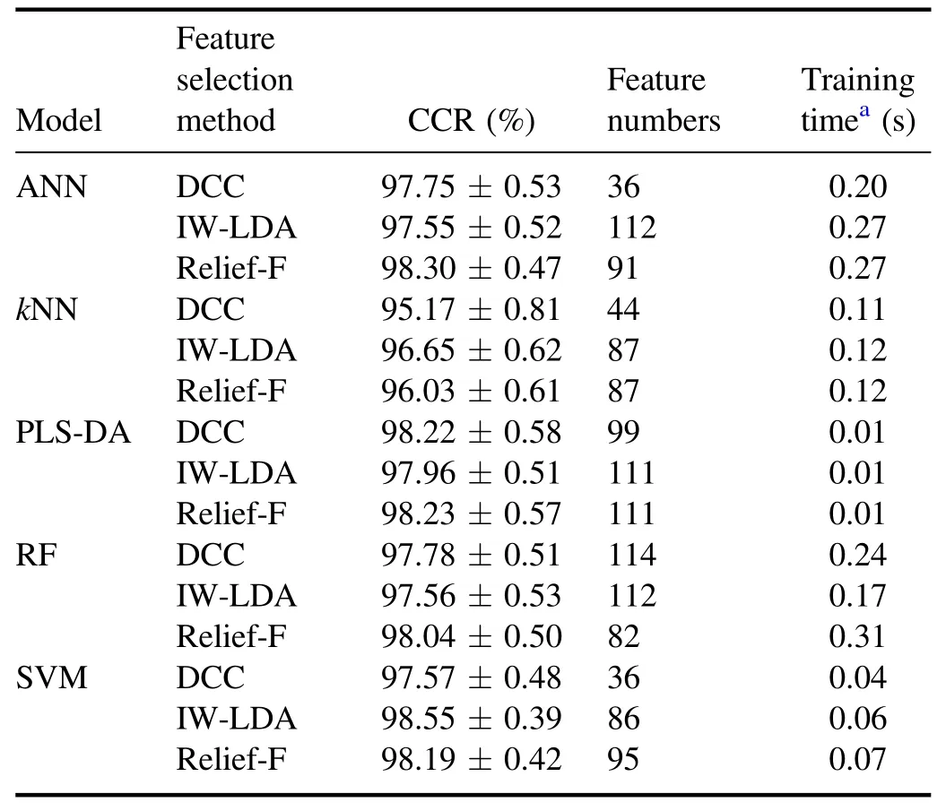
Table 4.The CCRs, feature variables numbers, and time complexities of all models.
The DCC method sorts the feature lines according to the correlation between lines and labels.The first feature line, C 819.6 nm in this case, has the highest correlation coefficient.Therefore,when using only one feature line,all classification models with the DCC method achieve the highest CCR.Meanwhile, for all models except RF, the optimal number of feature variables selected by the DCC method is the lowest compared to IW-LDA and Relief-F.The IW-LDA method sorts the feature lines by evaluating the contribution of variables on data diversities between the different wood species directly in the process of dimension reduction.The projection eigenvalues of LDA can separate different classes of data as much as possible.The Relief-F method sorts the feature lines according to the discrepancy between the different wood species directly in the process of analysis.This method selects out the nearest data in the same class and the other classes as near-hit and near-miss, respectively.The corresponding important weight of the variable is assessed by calculating the Euclidean distance between near-hit and near-miss, which represents the discrepancy between different classes.However, the diversity information between the data from different species is more prominent only when using sufficient feature lines.Hence, for most models, the optimal feature number selected by Relief-F and IW-LDA is more than that selected by the DCC method.It should be pointed out that these feature selection methods used supervised information,therefore the improvements of the CCRs of the classification models based on these methods are reliable only when the number of training data is large and the corresponding distribution information of the wood species is real and enough.
In summary, the results indicate that with the aim of obtaining a classification model established by a few variables(considering reduced model complexity), the DCC method might be a suitable one.With the aim of improving modelCCR, IW-LDA and Relief-F might be suitable feature selection methods for the classification task of wood species.

Table 5.The optimal parameters of all models corresponding to the optimal CCRs.
5.Conclusions
The LIBS technique is used to classify eight types of wood species (African rosewood, Brazilian bubinga, elm, larch,Myanmar padauk,Pterocarpus erinaceus, poplar, and sycamore) based on five classification models (ANN,kNN, PLSDA, RF, and SVM) combined with the feature selection methods in this paper.The spectral data are normalized by the maximum of data.DCC, IW-LDA, and Relief-F methods are used to select the feature variables by assessing the important weight.The classification models are established by training set data and the parameters of the model are optimized by 10-fold cross-validation.The CCRs of these five models are used as criteria to evaluate the performance of these three methods.
The CCRs of models built based on the different number of feature variables (according to the important weight) are obtained and compared.The experimental results show that the highest CCR is(98.55...0.39)%when the SVM is selected as the classification model (the corresponding variables number is 86 for the IW-LDA method).Comparing all results,DCC might be a suitable feature selection method considering reduced model complexity.With the aim of improving model CCR, IW-LDA and Relief-F might be suitable feature selection methods for the classification task of wood species.The results demonstrate that some simple and effective feature selection methods could improve the recognition ability of machine learning models for wood materials from LIBS data.In our future research,LIBS will be applied to analyzing and investigating the region of origin of wood.
Acknowledgments
The authors gratefully acknowledge support from National Natural Science Foundation of China (No.62075011) and Graduate Technological Innovation Project of Beijing Institute of Technology (No.2019CX20026).
 Plasma Science and Technology2021年5期
- Plasma Science and Technology的其它文章
- Programmable electron density patterns induced by the interaction of an array laser and underdense plasma
- Study of the tungsten sputtering source suppression by wall conditionings in the EAST tokamak
- Explicit structure-preserving geometric particle-in-cell algorithm in curvilinear orthogonal coordinate systems and its applications to whole-device 6D kinetic simulations of tokamak physics
- Comparison between fluctuation of floating potential gradient and velocity of blob structure on HL-2A tokamak
- Magnetic diagnostics for magnetohydrodynamic instability research and the detection of locked modes in J-TEXT
- Dielectric breakdown properties of Al-air mixtures
