Haitao Liao

1 Introduction

Systems encountered in practice generally exhibit some amount of nonlinear behavior.Nonlinearity introduces phenomena including amplitude dependant response frequencies,sub- and super- harmonic responses, and multiple stable responses to a given excitation[Nayfeh and Mook (1979); Neild, Champneys, Wagg et al. (2015); Dai, Wang and Schnoor (2017)]. Yet more complexity emerges when multiple Degrees of freedom (Dof)are present, because the superposition principle that greatly simplifies the decomposition of linear problems cannot hold for nonlinear systems.

Common tools for performing dynamical analysis of elastic structures are the Nonlinear Normal Modes (NNMs) for free vibration problems and the nonlinear frequency response curve for forced vibration problems. NNMs can be regarded as the extension of the concept of linear normal modes to nonlinear systems. Rosenberg [Rosenberg (1959,1966)] first defined NNMs as certain synchronous oscillations exhibited by the conservative nonlinear equations of motion. Inspired by the center manifold technique,Shaw et al. [Shaw and Pierre (1991); Shaw (1994)] constructed the NNMs by introducing two dimensional invariant manifolds for both conservative and non-conservative system.Recently, periodic orbits of nonlinear dynamic systems are viewed as the nonlinear normal modes, which give theoretical and mathematical tools for performing mode analysis of nonlinear structures.

Many nonlinear continuous or multi-degree of freedom systems exhibit some particularly novel responses whenever one mode of free vibration has a natural frequency that approaches an integer ratio to that of another, a condition known as internal resonance.The internal resonances have strong energy dependence on the oscillation frequency of the corresponding NNMs.

The nonlinear phenomena of modes coupling and internal resonances have been intensively investigated for nonlinear structures. For example, Nayfeh et al. [Nayfeh and Mook (1979)] conducted the research works of the analysis of nonlinear oscillators with modal interactions and multi-degree-of-freedom system with internal resonance. Using an L-shaped piezoelectric structure with quadratic nonlinearity, Cao et al. [Cao, Leadenham,Erturk (2015)] showed exploitation of its two-to-one internal resonance increased significant frequency bandwidth compared to its 2-DOF counterpart. Ghayesh et al.[Ghayesh (2011); Ghayesh, Kafiabad, Reid (2012)] discussed the internal resonances by using a numerical approach. Sze et al. [Sze, Chen and Huang (2005)] studied the sub- and super-harmonic resonance under the internal resonance condition of a translating strip by using the incremental harmonic balance method. Kerschen et al. [Kerschen, Peeters,Golinval et al. (2009); Peeters, Viguié, Sérandour et al. (2009) defined NNMs as the periodic motions of nonlinear systems and developed numerical iteration continuation techniques for NNMs. Goncalves et al. [ Gon?alves and Del Prado (2004)] studied the effect of non-linear modal interaction on the dynamic instability of cylindrical shells under axial loads. Hill et al. [Hill, Cammarano, Neild (2015)] applied the backbone curves to study internal resonance phenomena in systems of coupled nonlinear oscillators. Arvin et al. [Arvin and Bakhtiari-Nejad (2013)] investigated nonlinear modal interactions in rotating composite Timoshenko beams and considered the nonlinear coupling of transverse, shear and longitudinal motions. Amano et al. [Amano, Gotanda and Sugiura (2013)] analyzed internal resonances of a flexible rotor supported by a magnetic bearing. More detail on this topic can be referred to Renson et al. [Renson, Kerschen, Cochelin (2016)].

Identification of severe mode localization in the design process can help prevent failure due to High Cycle Fatigue (HCF) in periodic structures such as turbine blades. Many efforts have been devoted to the study of localization phenomena of bladed disks. For example, Chen et al. [Chen and Shen (2015)] provided useful mathematical insights into linear mode localization in nearly cyclic symmetric rotors with parameter uncertainty.However, this study deals with the mode localization of linear bladed disks. For nonlinear bladed disk, mode localization is unavoidable. By virtue of the continuation technique and the shooting method, Georgiades et al. [Georgiades, Peeters, Kerschen et al. (2009)]investigated the NNMs of periodic structure with cubic nonlinearity. Some of the recently works on the localization of nonlinear periodic structures can be found in Grolet et al.[Grolet, Hoffmann, Thouverez et al. (2016); Papangelo, Grolet, Salles et al. (2017)].

There have been some studies on the literatures that propose gradient based optimization methodologies to solve nonlinear dynamic problems [Liao (2014); Coudeyras, Sinou and Nacivet (2009); Liao (2015)]. In an earlier work [Liao and Sun (2013)], a hybrid approach combining the harmonic balance method and Sequential Quadratic Programming (SQP) method is employed to determine the worst resonance response of nonlinear systems. Under the nonlinear equality constraints which are constituted from the corresponding system of harmonic balance equations, the unknown Fourier coefficients and vibration frequency are optimized simultaneously. In Liao et al. [Liao(2015)] as a continuation of Liao et al. [Liao and Sun (2013)], the constrained optimization harmonic balance method is extended to solve the fractional order nonlinear systems and a general formulation for operational matrix of multiplication for polynomial nonlinearity is achieved.

It is clear that considering the Fourier coefficients as optimization variables, the optimization problem would become much more difficult as the size of optimization problem grows. With respect to the large number of variables and constraints, the use of SQP method is very costly or even impossible, due to the fact that gathering second order information for the approximation of the Hessian matrix could be an insuperable task. In generally, the constrained optimization harmonic balance method is not suitable for solving large size optimization problems. Therefore, an adequate treatment of the large system of nonlinear equality constraints is required, which motivates the search for new approaches with considerably lower computational cost.

The development of more realistic and efficient optimization technique has been the focus of extensive research efforts. The application of reduced SQP method to more general optimization problems is a viable way to tackle large scale optimization problems0. For typical nonlinear dynamics applications, the nonlinear optimization problem may have several thousand variables, but only relatively few degrees of freedom according to the number of control parameters. This makes the reduced SQP method a suitable candidate for solving large scale optimization problems. For example, a reduced Hessian method is developed in Biegler et al. [Biegler, Nocedal, Schmid et al. (2000);Biegler, Nocedal and Schmid (1995) for large scale constrained optimization problem. In Schulz et al. [Schulz and Book (1997)], the partially reduced SQP m0ethod is devoted to design the shape of turbine blades. Motivated by the above discussion, the reduced SQP method is exploited in this paper to solve the worst resonance response problem. To the best of author’s knowledge, there seems to be no contributions on the harmonic balance method considering the reduced SQP method.

The rest of the paper is organized as follows: In Section 2, the nonlinear constrained optimization problem and its sensitivity gradients are formulated. The process of reducing the original nonlinear equality constraints optimization problem to the simple boundary constraints optimization problem is described in detail. Typical numerical simulations are implemented in Section 3 to validity the present method. In Section 4,nonlinear mode analysis of nonlinear cyclic structure is conducted via the proposed method. Finally, the paper is concluded in Section 5.

2 The proposed method

This section gives a formal statement of the reduced space harmonic balance method.With the nonlinear equality constraints derived from the harmonic balance method, the formulation and implementation of the reduced SQP method used for solving the nonlinear constrained optimization problem is presented.

2.1 System equation of motion

The general equation of motion of nonlinear systems withnDof is expressed as

where M, D and K represent the mass, damping and stiffness matrices, respectively.,are the displacement, velocity and acceleration of the structure andrepresents the vector of nonlinear effects in the system and p(t) is the vector of the external forces.

2.2 Optimization problem formulation

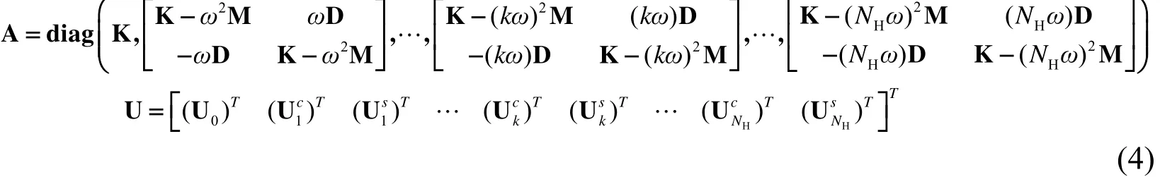
Based on the harmonic balance method, the unknown periodic displacement is expressed as a truncated Fourier series truncated at an orderNHselected.

whereare the cosine and sine coefficients of thekth harmonic,respectively.

The substitution of Eq. (2) into Eq. (1) results in the following algebraic equation:

wherecorresponds to the Fourier coefficients of the nonlinear forcing term and the external force;respectively defined by

In order to evaluate the term, the Alternate Frequency/Time(AFT) domain method is used. This method consists in evaluating the nonlinear forces in the time domain over a period and computes the discrete Fourier transform to obtain its influence in the frequency domain. This process is shown in the form of a flowchart in Eq. (5).

where FFT and IFFT represent the Fourier transform and its inverse operation,respectively.

To improve the computational efficiency related to the Fourier transform operation, the following relationship can be utilized for the polynomial nonlinearity0

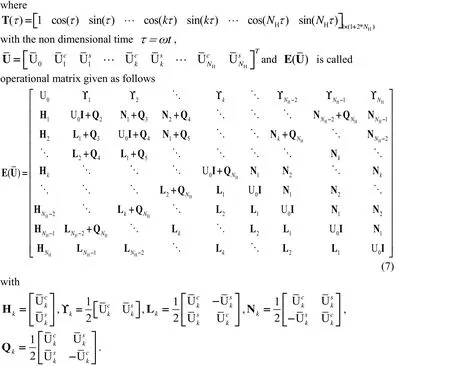
Following the recursive procedure expressed in Eq. (6) the Fourier coefficients of the polynomial nonlinear terms are obtained analytically, leading to a significant reduction in computational time.

Since the Fourier coefficients and vibration frequency are considered as optimization variables in the framework of the constrained optimization harmonic balance method[Liao and Sun (2013); Liao (2015)], the nonlinear equality constraints must be imposed in the optimization problem which can be stated as follows:

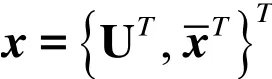
where.The vibration frequency and system parameters and/or uncertainty parameters can be included inrepresents the nonlinear equality constraints. Inequality constraintsrefer to lower bound and upper bound specifications.

The iterative process of the gradient optimization algorithm requires the sensitivity analysis of the nonlinear optimization problem. Therefore, sensitivities (gradients) of the objective and constraint functions with respect to the optimization variables are required.

For the AFT method , the termin the Jacobian matrix of the nonlinear equality constraints takes the form

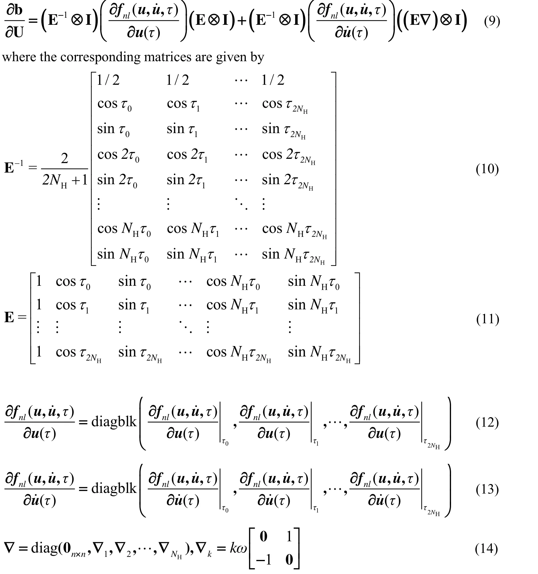
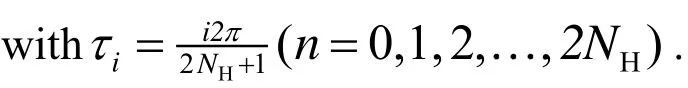
If the analytically expression in Eq. (6) is used for polynomial nonlinearity, the gradient ofis given in Eq. (14) of [Liao (2015)].

The sensitivity of the nonlinear equality constraints with respect tocan be derived easily. By incorporating these gradient formulas into a gradient based optimization method, the nonlinear programming problem can be solved.

Tackling problem in Eq. (8) is quite challenging due to the relatively large number of variables and constraints. Therefore, further actions should be taken. In this work, the solution to the optimization problem stated in Eq. (8) is accomplished by using the reduced SQP algorithm.

2.3 The reduced Sequential Quadratic Programming method for solving the constrained optimization problem

A short introduction to the reduced SQP approach will be provided for completeness. The SQP method which is well-suited to solve the constrained optimization problem in Eq.(8) can be considered as extensions of quasi-Newton methods taking constraints into account. It solves Eq. (8) iteratively by improving the current iterate. An updateis calculated by making a linear approximation of the constraints and a quadratic approximation of the gradient of the Lagrangian, whereis the Lagrangian multiplier. The quadratic programming subproblem can be described as:

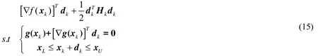
in whichis the Hessian of the Lagrangian function. The symboldenote gradients with respect to the optimization variableis used to

For dynamic optimization problems, the dimension of state variables is generally much larger than that of control variables. In order to obtain a simpler optimization problem,the gradients of nonlinear equality constraints can be exploited to simplify the optimization problem in Eq. (15). According to the reduced SQP method, the tangent space of the nonlinear equality constraints is divided into range space and null space. The search directionis decomposed in a range space solutionand a nullspace solution

It is clear that the success of decomposition methods relies on a wise choice of the reduced basis. Three techniques have been developed to build the reduced basis. The use of orthonormal basis for the space decomposition is first investigated. However, this decomposition scheme involves expensive QR factorization. To avoid the expensive computational cost for QR factorization, alternative numerical techniques such as orthogonal basis and coordinate basis methods have been proposed. Orthogonal basis and coordinate basis methods rely upon the gradients of nonlinear equality constraints in Eq. (15).

On the basis of the null space technique,is represented with the combination of the range space solutionand the null space solution:

whereconsists of the range space basis matrix whileis related to the null space basis matrix. The matrixsatisfies the relationship

The reduced SQP method relies on the matricesandsuch thatis square and full rank. The derivatives of the nonlinear equality constraint define the null space and the range space related matrices. For the decomposition method related to the orthogonal basis, the most popular choice ofandis built as

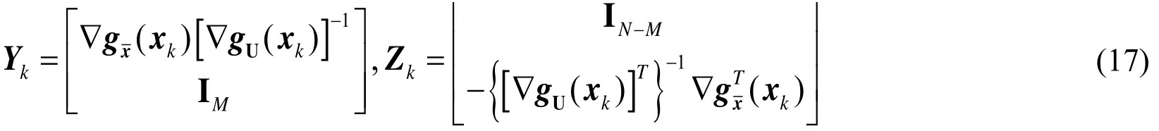
whereNis the number of optimization variables andMrepresents the size of the nonlinear equality constraints.

In the case of the coordinate basis decomposition method, the basis matrixin the null space is the same as in Eq. (17) while the basis matrix in the range space is replaced by

Given the particular selection ofandin Eq. (16), the range space solution for Eq. (15) is determined by. Note that the invertibility oflows from the non-singularity of the Jacobian matrix of harmonic balance equations, which is a required condition for the construction ofand the solution of. For some occasions, the Jacobian matrix may become singular. However,the application of the reduction techniques requires the Jacobian to be non-singular. To overcome this drawback, the basis change is adopted in this paper. The reader may consult [Biegler, Nocedal, Schmid (2000); Biegler, Nocedal and Schmid (1995)] for a detailed discussion about the basis change.

By inserting Eq. (16) into Eq. (15) and utilizing the coordinate basis decomposition scheme with the propertythe following reduced space optimization problem is resulted:

Obviously, the nonlinear equality constraints are eliminated in Eq. (19). The originalNdimensional quadratic subproblem in Eq. (15) has been replaced by aN-Mdimensional quadratic subproblem expressed in Eq. (19). It is very beneficial to the reduction of the computational complexity and the improvement of calculation efficiency.

To accomplish the optimization iteration in accordance with Eq. (19), the cross termand the reduced Hessian matrix are needed. It should be noted that the calculation ofincurs a substantial computational burden. In order to avoid the need to compute the cross termat every iteration,s replaced by an approximation matrixand the vectoris calculated. For every iteration, the approximation matrixs updated with the expression proposed by Broyden:

where the vectors

The BFGS algorithm which can iteratively calculate a better approximation to update the reduced Hessian matrix is adopted as follows

Based on the calculated cross term and reduced Hessian matrix, Eq. (19) can be solved forand thuscan be obtained. Finally, the updateis assessed by a globalization strategy which enforces convergence to the optimization solution regardless of the quality of the initial solution guess.

Aline-search of the globalization strategy is performed to find a new iterate withbeing the step length which provides a sufficient decrease of the merit function

where the penalty coefficientis chosen large enough to ensure thatis a descent direction for

By virtue of a one dimensional optimization technique, the step lengthis iteratively determined based on a sufficient decrease condition, i.e. the so-called Armijo condition[Wright and Nocedal (1999, 2006a)]:

whererepresents the directional derivative for the merit function. For the direction, the directional derivative is given by

Additional details of the reduced SQP technique can be found in the Refs. [Wright and Nocedal (1999, 2006a, 2006b)].

The key features of the proposed work are the use of harmonic balance principle within the constrained optimization framework and the suitability for handling nonlinear equality constraints exploiting the reduced SQP method.

3 The validation of the proposed method

In this section, three numerical examples which have been taken from recent publications are implemented to verify the effectiveness of the proposed method. The equation of motion is given by:

where overdot denotes the differentiation with respect to time.Fis the forcing amplitude andis the frequency of the external excitation.,andare the mass, damping and stiffness coefficients, respectively.denotes the cubic nonlinear coefficient.,are the coefficients of the fractional derivative terms with the ordersp1andp2,respectively.

From an engineering view point, the Caputo definition for fractional derivative is adopted and defined as follows:

In this paper, the fractional derivative is considered in the frequency domain using the expression in Eq. (3) of Liao [Liao (2015)]. The interested reader is referred to the aforementioned paper for further details about the fractional differentiations.

3.1 Numerical results for the Duffing oscillator

For a first demonstration of the methodology, a Duffing oscillator is considered. The Duffing model is an example of dynamical systems that exhibit nonlinear behavior. The model is used with the following parameters:=0,F= 0.1. The structural parameters are taken from an example in Eq. (2) of Wang et al.[Wang and Zhu (2015)].

In order to demonstrate the feasibility of the proposed algorithm, a continuation technique is used to get the reference numerical solutions for comparison. The continuation of the periodic motion is accomplished by the pseudo arclength continuation method. In the numerical computations, only the first five harmonics are retained in the Fourier expansion of the response. The frequency response curves are depicted in Fig. 1 where solid and dashed lines represent stable and unstable periodic solutions,respectively. In Fig. 1,Hidenotes theith harmonic. It can be seen from Fig. 1 that the system reaches the top amplitude at resonant frequency=1.6545.

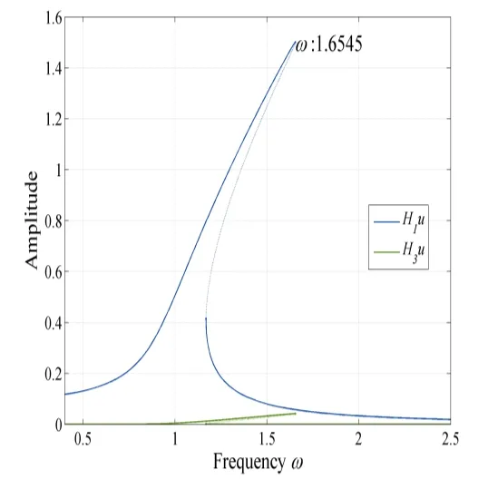
Figure 1: The frequency response curves of the Duffing oscillator

The resonant peak in Fig. 1 is searched by utilizing the proposed method. The vibration displacement is maximized. The unknown variables that have to be determined are the unknown Fourier coefficients and the resonant frequency of the worst case resonance response. The excitation frequency is considered to be independent optimization variable which is suitable for nonlinear optimization analysis. The optimization is conducted by retaining only 5 harmonics of the temporal response of the structure. The initial guess of the frequency is set toThe maximum number of iterations is set to 500 under the convergence tolerance of 10-8. A smaller tolerance will lead to a higher precision, but more iterations are required meanwhile.

A convergence curve is ended, after the corresponding algorithm finds the optimal solution or the termination condition is satisfied. The L1norm of the nonlinear equality and inequality constraints is used for the convergence criteria. To provide an intuitive illustration, Fig. 2 plots the convergence processes of the proposed algorithm. In Fig. 2,the results tend to converge after 101 generations and additional generations will not produce better solutions.

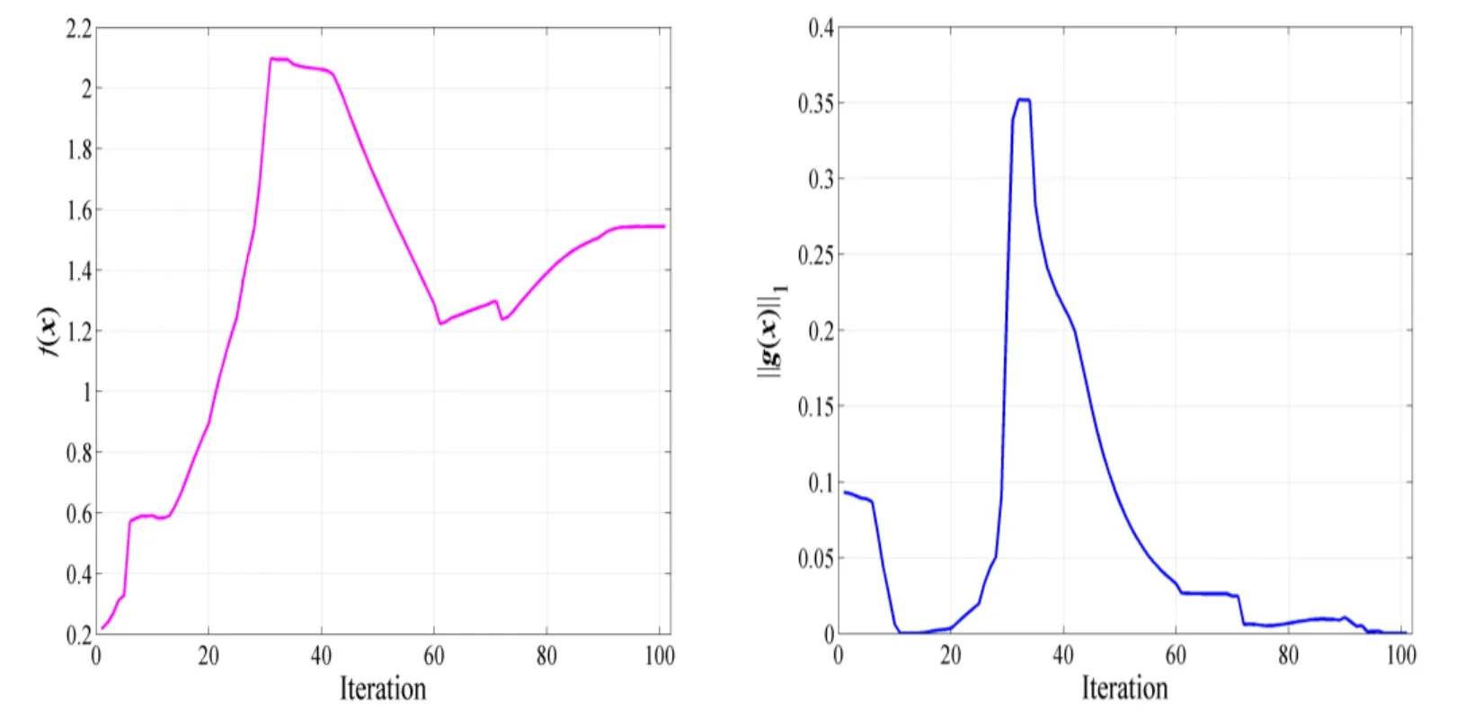
Figure 2: Evolution of the optimization algorithm

A direct comparison of the numerical results between the two methods for the peak solution is presented in Fig. 3. As shown in Fig. 3, there is one main harmonic term in the system response and the presence of several higher harmonic components can be detected.Moreover, the harmonic coefficients associated with even harmonics are zero. Observe in Fig. 3 that the peak solutions obtained from both the proposed method and the continuation method are verified to be in a good agreement although minor discrepancy remains.

Figure 3: Numerical optimization results of the Duffing oscillator obtained by the proposed method

In order to fully validate the present approach, direct numerical integration has been carried out for the peak solution. The initial conditions can be readily supplied by the results of the presented method. The portrait for the worst case response solution is presented in Fig. 4 using the time integration method (denoted by TI) and the proposed method (denoted by RSHBM). From Fig. 4, it is evident that the present approach solution matches well with the numerical integration solution. Therefore, the validity of the presented method is confirmed.

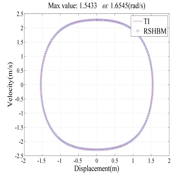
Figure 4: The comparison of the phase portrait for the peak solution between the time integration method and the proposed method

3.2 Numerical results for the fractional Duffing oscillator

The second example is selected from Eq. (1) of Shen et al. [Shen, Wen, Li et al. (2016)].Three cases are investigated by utilizing the proposed method. The values of the system parameters are listed in Tab. 1.

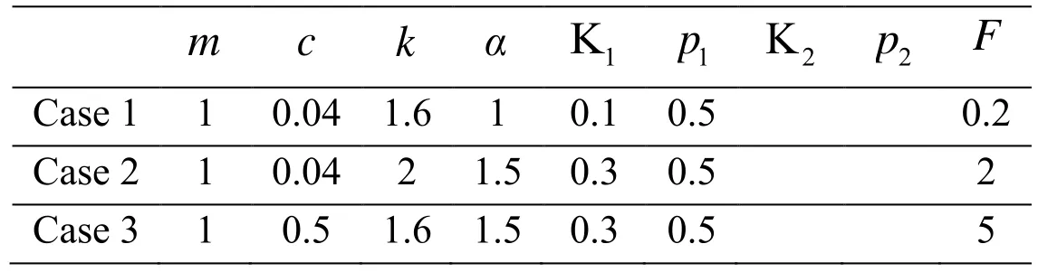
Table 1: The selected parameter sets

The resonance peak response can be found by using the numerical continuation method.Fig. 5 shows the continuation frequency response curves for the three cases given in Tab.1. Observe in Fig. 5 that not only major resonances occur, but also super harmonic resonances are detected. Although the response curves for the three cases are roughly in similar shape, the curvatures and turning points are different. Case 1 results in relatively weak nonlinear behavior. The highest amplitude for case 1 is around=1.6962. For case 2, the vibration amplitude achieves the maximum value 3.5307 and the peak frequency is located at= 3.9911. The maximum displacement for case 3 occurs close to=3.0841.

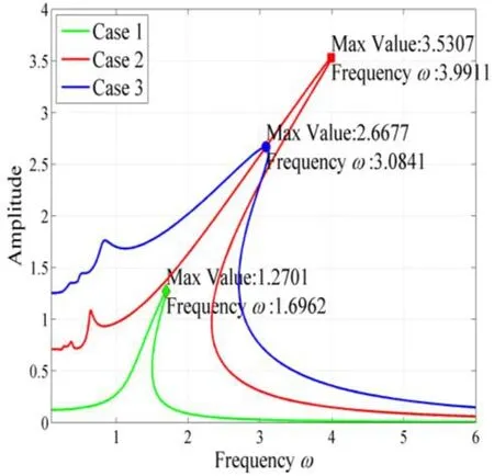
Figure 5: The frequency response curves of the fractional Duffing oscillator for the three cases

The proposed reduced SQP algorithm is implemented to find the peak solution which satisfies the harmonic balance constraints to a sufficient degree of accuracy and efficiency.The tolerance is set to be 10-8. The convergence histories of the objective function and the L1norm of the nonlinear constraints are shown in Fig. 6. As illustrated in Fig. 6, the peak solutions converge reasonably well within 100 iterations. The iteration numbers for cases 2 and 3 are 76 and 35 times respectively, as shown in Fig. 6(b) and 6(c).

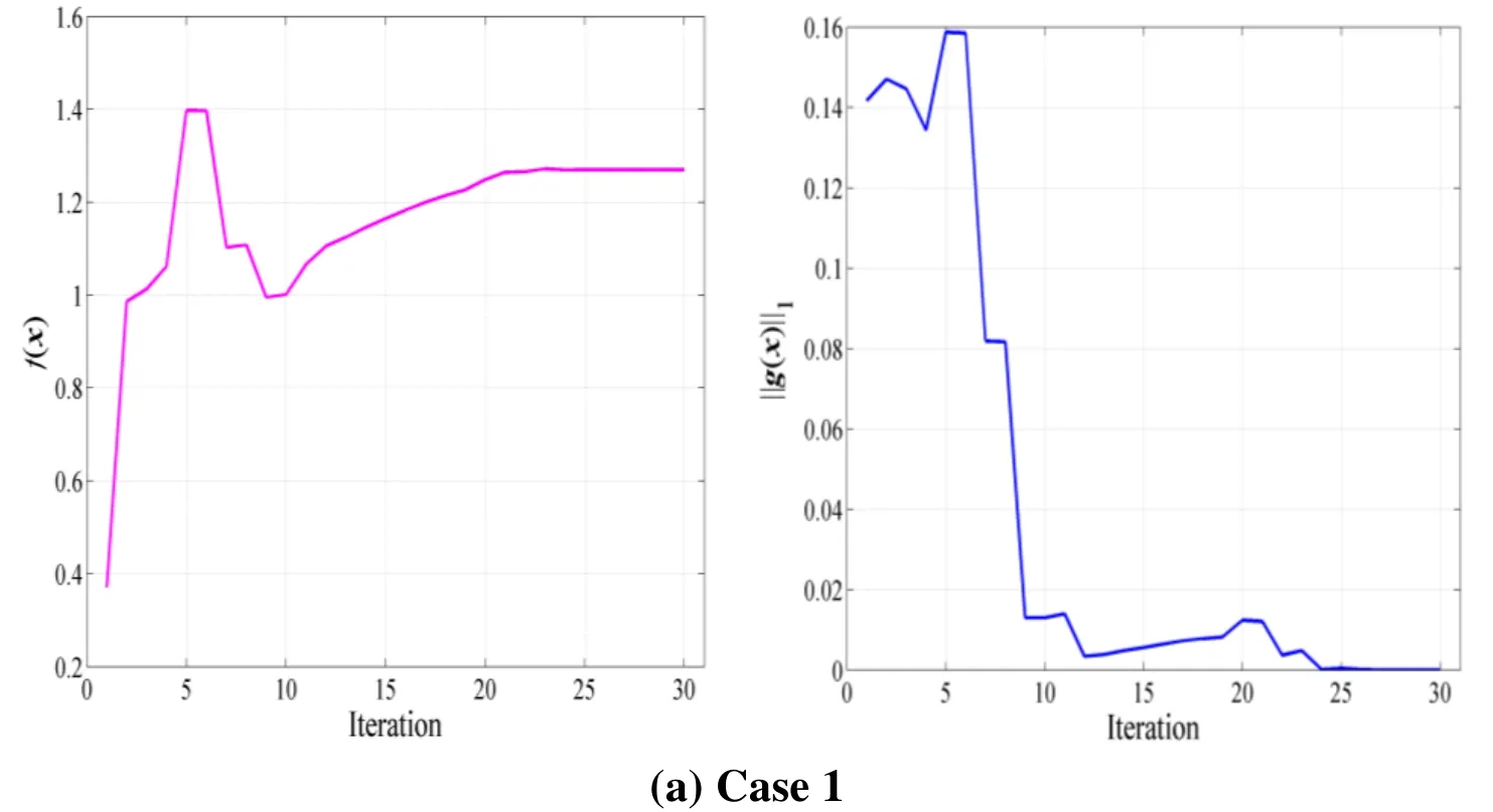
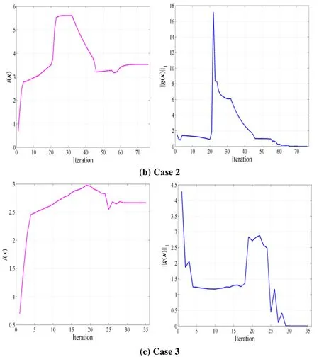
Figure 6: Evolution of the objective and constraint functions

Based on the proposed method, the optimization results together with the peak solutions of the continuation method are summarized in Fig. 7 for the three cases. As can be seen in Fig. 7, the first harmonic component is the strongest component in the total response and the values of the other harmonic terms are much smaller than the values of the first harmonic term. The harmonic components calculated with the present method reproduce the reference solutions from the continuation method.

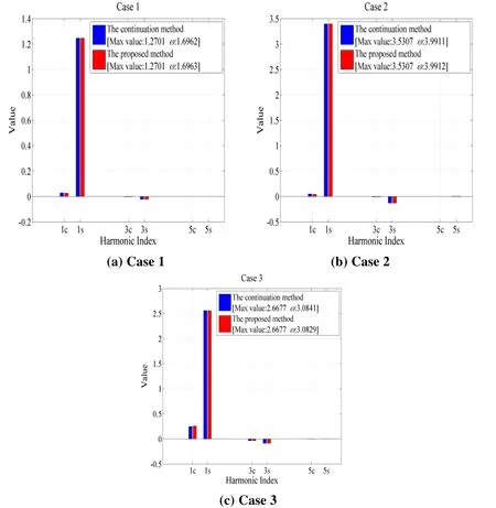
Figure 7: The optimization results for the fractional Duffing model

For case 1, the optimization simulation predicts a maximum amplitude of 1.2701 at=1.6963. A maximum vibration amplitude of 3.5307 for case 2 is found at=3.9912.For case 3, the predicted worst resonance response occurs at=3.0829 and the maximum vibration amplitude is up to 2.6677. In comparison with the top resonance in Fig. 5, the resonance frequencies as well as the resonance amplitudes calculated by the present method agree well with the results obtained the conventional continuation method. The results of the present method have satisfactory accuracy.

3.3 Numerical results for the Duffing oscillator with two kinds of fractional derivative terms

The third example considered is a fractional order Duffing system with two fractional order derivative terms. This example is borrowed from the author’s previous work. Tab. 2 which is taken from Tab. 8 of Liao [Liao (2015)] furnishes an overview of the main parameters used for the numerical model.

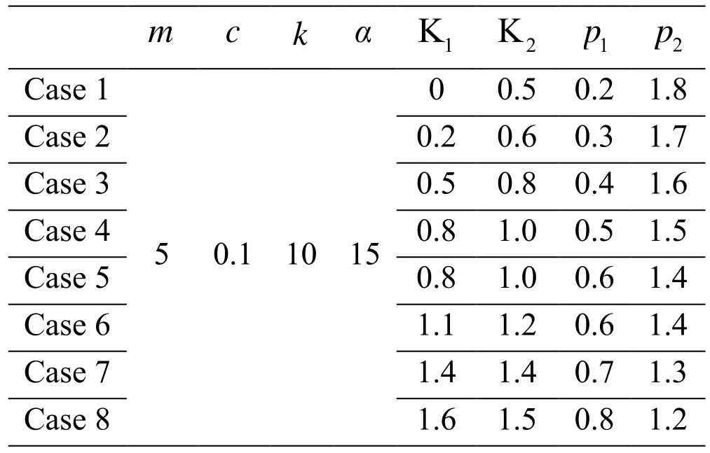
Table 2: The numerical simulation parameters

The optimization results with the proposed method are presented in Tab. 3 where the iteration numbers are presented in the second column. From Tab. 3, it can be easily observed that the reduced SQP method is more robust and has stable iteration numbers.For all cases, the proposed method can produce the convergent solutions less than 100 iterations. When compared with the published reference solutions given in Tab. 9 of Liao[Liao (2015)], good agreement is achieved although slight discrepancies are observed.The agreement of comparison between the proposed method and the benchmarks indicates that the resonance peaks are captured well by the proposed method and the present analysis is accurate. The validity of the present method is verified.

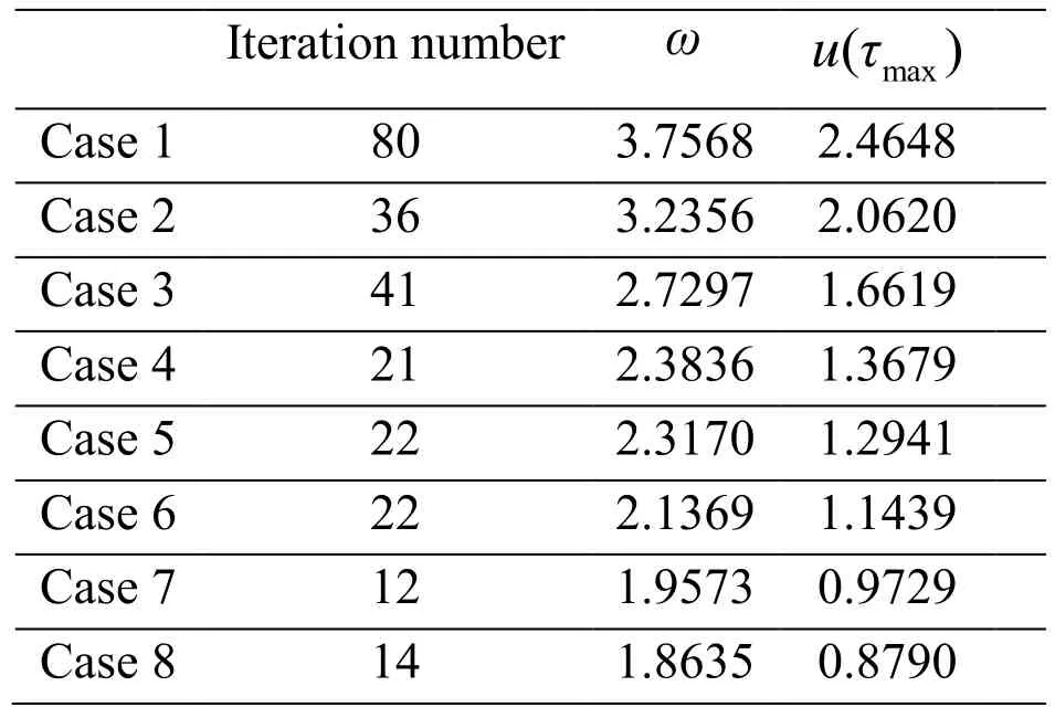
Table 3: Summaries of numerical analysis results

In all these examples considered, the solutions obtained from both the conventional continuation method or other researches in the literature and the proposed method are verified to be in a good agreement. The simulations show that the reduced SQP algorithm has good global convergent ability and can quickly converge to the global optimal solution with few iteration.

4 NNMs of the bladed disks with geometrical nonlinearity

The proposed algorithm for several examples against the standard continuation method is verified. In the following section, the present approach is utilized to perform nonlinear modal analysis of periodic structures.

4.1 The two-Dof-per-sector model

The numerical application example is inspired from Georgiades et al. [Georgiades,Peeters, Salles et al. (2009)]. The system is a simplified mathematical model of a bladed disk assembly.A periodic structure with 30 substructures is considered. A sector of the model used in the analysis is shown in Fig. 8. Each sector is modeled using disk (M) and blade(m) lumped masses, coupled by linear (k) and cubic (knl) springs. The nonlinear springs can be representative of geometrically nonlinear effects in the blades. The disk masses are connected together by linear springsK.

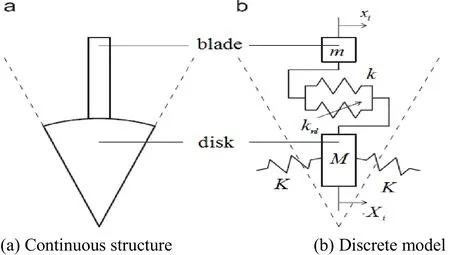
Figure 8: One sector of the system configuration and the corresponding discrete model

The motion equation of theith sector is described as follows:

whererepresent the blade and disk motion, respectively, for theith sector. The parameters of the system come from Georgiades et al. [Georgiades,Peeters, Salles et al. (2009)], and are given in the following:

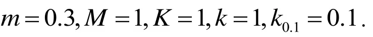
Natural frequencies of the tuned bladed disk without geometrical nonlinearity are given in Tab. 4 for all Nodal Diameters (NDs). As can be seen in Tab. 4, since the structure is not fixed, the first mode is a rigid-body mode, which is obviously not affected by the nonlinearities. In addition, due to cyclic symmetry of the structure, the bladed disk system possesses repeated eigenvalues.

Table 4: Natural frequencies of the underlying linear system

4.2 The localized NNMs

The proposed algorithm is used as the dynamic analysis tool to compute NNMs of nonlinear systems. A NNM is defined as a (nonnecessarily synchronous) periodic motion of the unforced conservative system. Due to the frequency energy dependence of nonlinear oscillations, NNMs are depicted in a frequency energy plot. In analogy with the frequency energy plot, the evolution of NNMs in this paper is presented in the frequency amplitude plot. In order to obtain the frequency amplitude curve, the vibration frequency is considered as the control parameter. The curve is obtained by varying the value ofwith a step length of 0.05 and calculating the extreme point numerically.

The proposed method is stepped up in the downward frequency sweep. The NNM initiates at the predicted localized solution at higher energy and continues to lower response amplitude as energy decreases. The first guess with localized solution predictor can be corrected using the proposed method. After finding the solution with a certain higher vibration frequency, the obtained periodic solution is used to define prediction for the next frequency decreasing point in the frequency amplitude curve. The periodic solution computed from the previous step is used as initial guess for the periodic solution in the next step so that the convergence of the iteration process can be improved. By repeating the same procedure, the frequency amplitude curve is constructed.

The frequency is tuned from 5 to 0 with a step of 0.05 Hz. The NNM initiates at=5 which starts as different harmonic component interaction. The amplitude frequency curve of the NNMs can be constructed by sequentially decreasing the vibration frequency and using the result of each step as the initial guess of the next point.

Using the new guess predictor, the response of the next step can be determined by the present method. The proposed method is applied to solve Eq. (8) for a given frequency. It uses a known periodic motion to identify the next solution and the maximum displacement is taken to be the objective function.

Figure 9: The localized NNMs with single harmonic component

The results as a function of amplitudes with respect to frequencies are presented in Fig. 9.It can be seen in Fig. 9 that only the first harmonic emerges. The NNMs are energy independent and the vibration amplitude decreases as the vibration frequency decreases.Moreover, the localized motion occurs when the frequency is greater than=2.5 where the slopes of the curves are deeper. Fig. 10 shows two NNMs at two frequencies. Observe in Fig. 10 that all the Dofs vibration synchronously. The NNM at=5 is severely localized, with the significant energy mainly limited to a single blade. The Fourier coefficients corresponding to NNMs in Fig. 10 are given in Fig. 11. It has been found that the Fourier coefficients in Fig. 11(a) are positioned symmetrically with respect to blade 1.

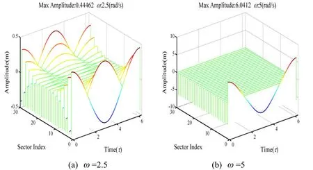
Figure 10: Modal response time histories at the two solutions

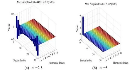
Figure 11: The Fourier coefficients for the solutions in Fig. 10

4.3 The case of 1:2 internal resonance NNMs

In this section, the NNMs corresponding to the internal resonance of type 1:2 are searched through the present method. The evolution of the NNMs as a function of the vibration frequency is presented in Fig. 12. Resembling the previous results, the vibration amplitude in Fig. 12 also monotonically decreases with decreasing the vibration frequency. The slopes of the curves are much deeper when the vibration frequency is small. The 1:2 harmonic interaction is recognized to take place at frequency greater than 2.5. The first and second harmonic components may interact with each other and energy exchange between these two harmonic contents exists. Decreasingweakens the nonlinear interaction due to the one to two internal resonance. The NNMs in the frequency range [1.25, 2.5] posses single harmonic motion. The first harmonic component vanishes asapproaches to 1.25.

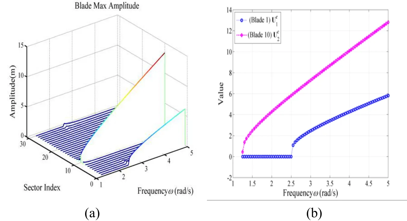
Figure 12: The amplitude variation with respect to

The time histories at three NNMs in Fig. 12 are shown in Fig. 13. In Fig. 13(b), the vibration energy is concentrated in blade 10. For the case 1:2 internal resonance in Fig.13(c), NNM at=5 is a localized NNM with high deformation around blades 1 and 10.Blade 10 oscillates at a frequency two times that of blade 1. Moreover, the response amplitude of blade 10 is nearly twice that of blade 1.

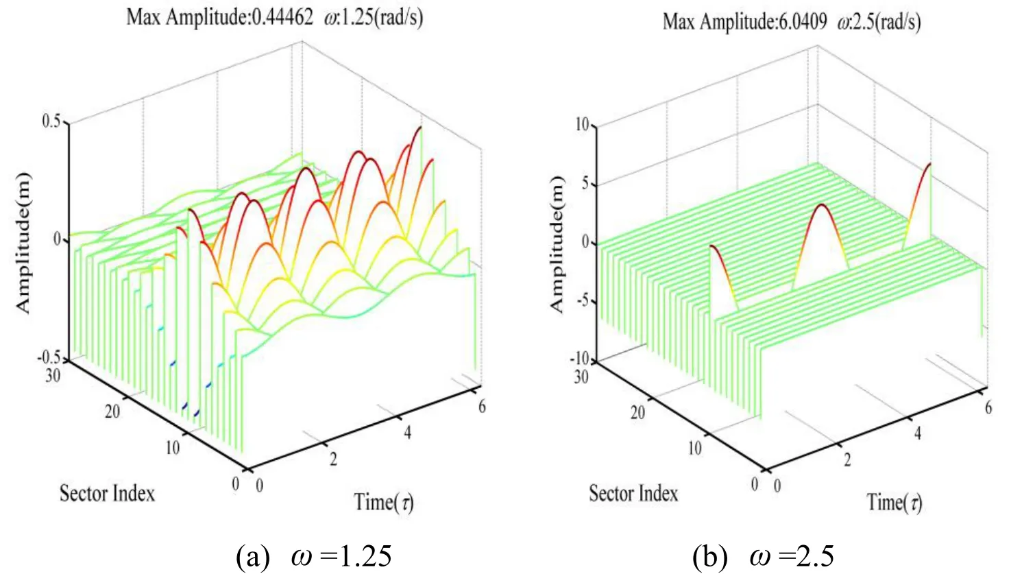
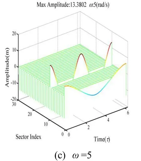
Figure 13: Time histories over a period motion for the three NNMs

The corresponding Fourier spectrums of these NNMs are given in Fig. 14. It can be seen in Fig. 14(a) that the Fourier coefficients are purely symmetric with respect to the localization blade. In addition, the NNM at=5 shows a significant contribution from the second harmonic component to the system response. A contribution from the first harmonic component is observed, but the contributions from the other harmonic components are negligible.

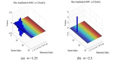
Figure 14: The Fourier coefficients related to the solutions in Fig. 13

4.4 The case of 1:2:3 internal resonance NNMs

The same strategy can be extended to study the NNMs of type 1:2:3 internal resonance.Fig. 15 depicts how the maximum amplitude of NNM changes in accordance with.Observe in Fig. 15 that as the frequency decreases from high values, the stable response amplitude decreases continuously. The response amplitude of the second and third harmonic contents is decreased more profoundly compared to the first harmonic component. However, the slopes of the curves are quite constant.

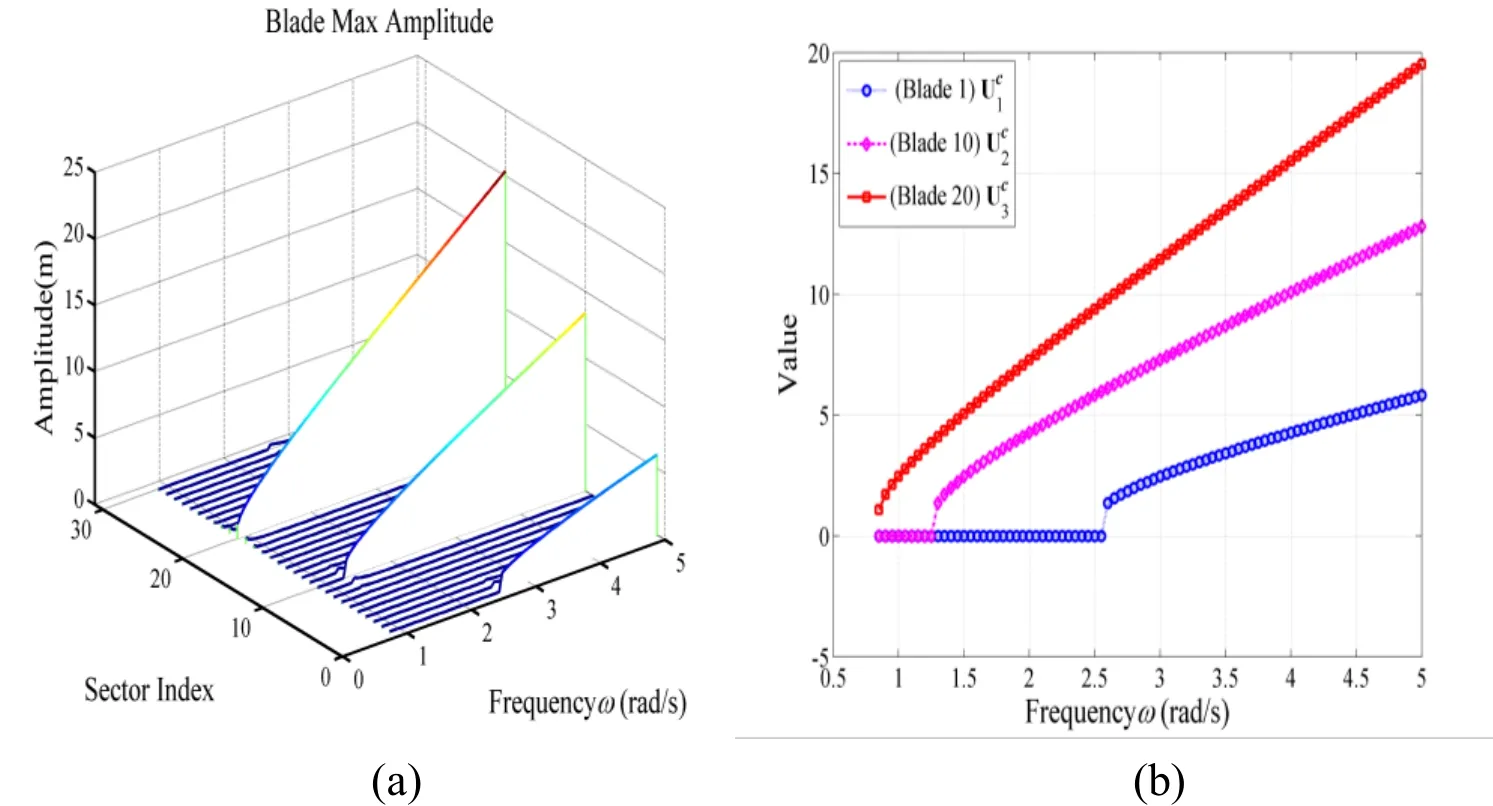
Figure 15: The NNM amplitude versus

In Fig. 25, 1:2:3 internal resonance is observed for a wide range of vibration frequency. A transition between 1:2:3 to 2:3 internal resonance takes place at=2.5. The two-tothree internal resonance between the second and third harmonic components is activated.

Nonlinear interactions are weakened with further decreases in. Beyond a certain frequency threshold, the second harmonic component disappears. Single-harmonic vibration is observed at frequency range from 0.85 to 1.25 and the sole third harmonic remains.

The time histories of the four NNMs are shown in Fig. 16. For NNM at=0.85, blade 20 will experience a much larger displacement relative to the other blades. Confinement of a significant magnitude of free response on blade 20 is observed in Fig. 16(b) at a frequency of 1.25. The localized NNM at=2.5 is evident in Fig. 16(c) where blades 10 and 20 oscillate with non-negligible amplitude. In Fig. 16(d), the vibration corresponding to NNM at=5 is confined mostly to three blade. The amplitude of blade 20 is nearly three times larger than that of blade 1.

The Fourier coefficients for the four NNMs in Fig. 16 are demonstrated in Fig. 17. In Fig.17(a), the response spectrum indicate that 3is the dominant frequency in the response and the obtained Fourier coefficients regarding the localized blade 20 are symmetric. The third harmonic component becomes more significant at higheras indicated in Fig.17(b). Considerable participation of superharmonic components (2, 3) is observed in Fig. 17(c). The numerical result in Fig. 17(d) shows a strong contribution to the structural response in terms of the third harmonic component with some interaction from the first and second harmonics.

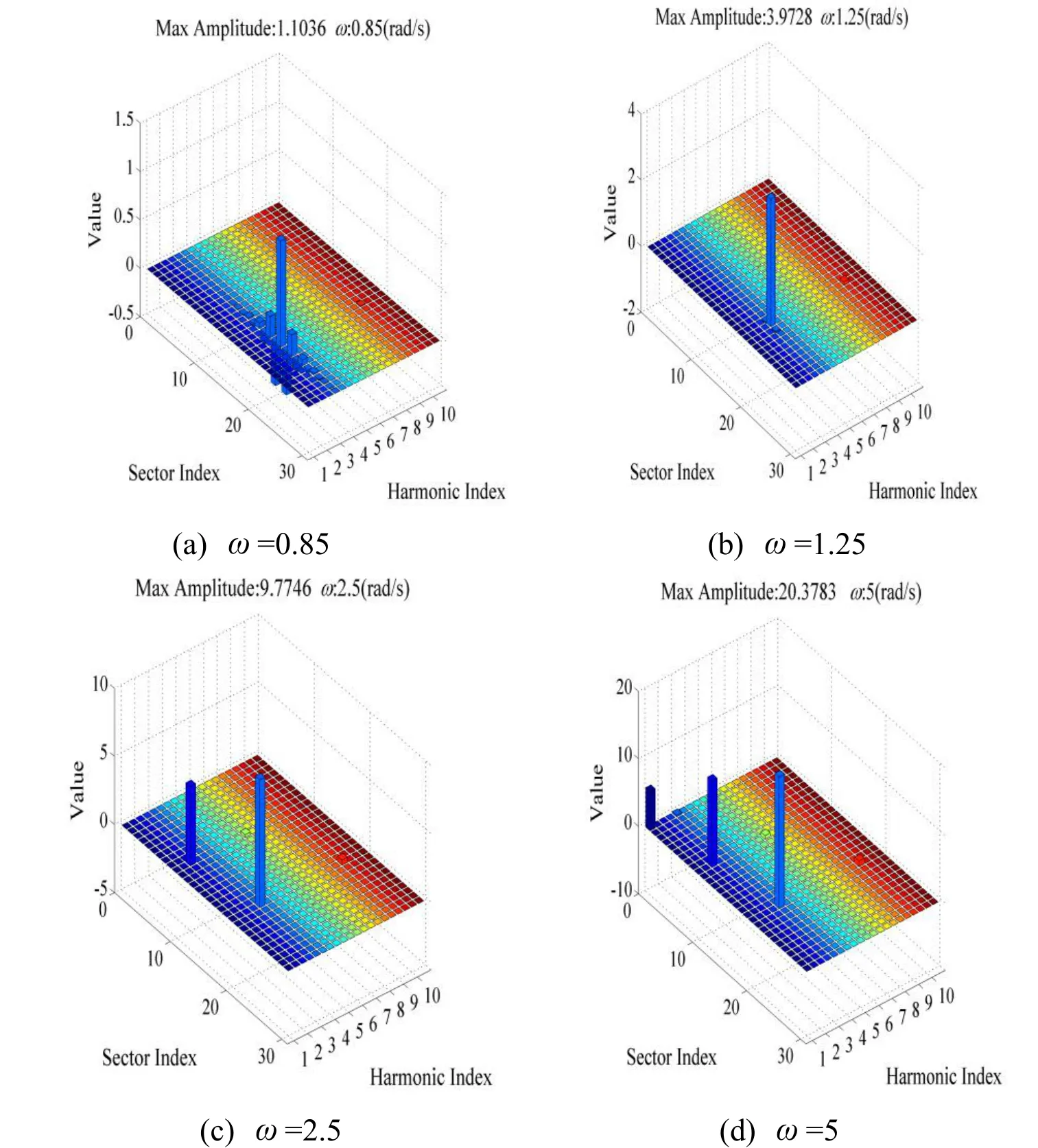
Figure 17: The Fourier spectra of the four NNMs in Fig. 16

The direct numerical integration of the dynamical system is carried out to confirm the exist of NNMs. The initial conditions for the numerical integration are obtained from the present method solutions. The system of differential equations is integrated over 1000 periods of vibration. The portraits for NNM at=5 are depicted in Fig. 18. It can be observed in Fig. 18 that the present method coincides with the time integration method well at=5 where stable response exists. Direct numerical simulation of the equations of motion indicates the NNMs at all frequencies are stable.

Figure 18: The comparison of the phase portrait of the NNM at =5 between the two approaches

The numerical results indicate that the proposed method can accurately predict different internal resonance NNMs. A infinity of periodic internal resonances exist for nonlinear bladed disk. Various types of the internal resonance could happen in cyclic nonlinear systems regardless of the commensurate condition of the eigenfrequencies of the underlying linear system. It is apparent that 1:1, 1:2 and 1:3 internal resonances are the special cases of the 1:2:3 internal resonance combination. All figures present quite similar type of amplitude frequency curve. The presence of harmonic component interaction with a strcit integer ratio of oscillating frequency violates the perfect condition of internal resonance. Due to the occurrence of separation, it is obvious that the continuation method is not able to capture some types of NNMs.

5 Conclusions

An approach which rests on the reduced SQP method combined with the harmonic balance method is proposed to search the localization nonlinear normal modes of various types of internal resonance. The proposed methodology includes two steps. The harmonic balance method is first employed to construct the nonlinear equality constraints for the constrained optimization problem. Then, the highly non-linear constrained optimization problem is solved by making recourse to the reduced SQP technique. The reduced optimization problem is formed by projecting the original optimization problem onto the null space basis which exploits the structure of nonlinear equality constraints. Therefore,the corresponding nonlinear equality constraints can be eliminated via the null space decomposition transformation and the simplified optimization problem subjected to bound constraints is established. Hence, the calculation process in the standard optimization iteration analysis becomes much simpler. The novelty of the approach described lies in the way in which the nonlinear equality constraints are removed.

The effectiveness of the proposed algorithm is demonstrated by several benchmark examples seen in the literatures. Simulation results demonstrate that the proposed algorithm has a fast convergence speed for finding the optimal solution. Nonlinear normal modes of nonlinear bladed disk are computed via the present method. It is shown that there is interaction between the harmonic components due to internal resonances and localization nonlinear normal modes of various types of internal resonances are detected.Higher order harmonics affect the system response more significantly. NNMs involving even harmonics are also observed for nonlinear systems with cubic nonlinearity. Another interesting phenomenon is that the Fourier coefficients of the localization NNM exhibit symmetry. It is worth mentioning that nonlinear modes with deformation localized to specific components of the structure appear. Localization can exist in the perfectly nonlinear symmetric structure, it does not dependent on the existence of parameter uncertainty or weak coupling between substructures.

Acknowledgements:The authors would like to thank the sponsor of the National Natural Science Foundation of China through grant No. 11502261, and the Aeronautical Science Foundation of China under award No. 2015ZB04002.The sponsor of the Beijing Institute of Technology Research Fund Program for Young Scholars is gratefully acknowledged by the authors.

Amano, R.; Gotanda, H.; Sugiura, T.(2012): Internal resonance of a flexible rotor supported by a magnetic bearing.International Symposium on Applied Electromagnetics& Mechanics, vol. 39, no. 1-4, pp. 941-948.

Arvin, H.; Bakhtiari-Nejad, F.(2013): Nonlinear modal interaction in rotating composite Timoshenko beams.Computers & Structures, vol. 96, pp. 121-134.

Biegler, L. T.; Nocedal, J.; Schmid, C.(1995): A reduced Hessian method for largescale constrained optimization.Siam Journal on Optimization, vol. 5, no. 2, pp. 314-347.

Biegler, L. T.; Nocedal, J.; Schmid, C.; Ternet, D.(2000): Numerical experience with a reduced Hessian method for large scale constrained optimization.Computational Optimization & Applications, vol. 15, no. 1, pp. 45-67.

Byrd, R. H.; Nocedal, J.(1990): An analysis of reduced Hessian methods for constrained optimization.Mathematical Programming, vol. 49, no. 1-3, pp. 285-323.

Cao, D.; Leadenham, S.; Erturk, A.(2015): Internal resonance for nonlinear vibration energy harvesting.European Physical Journal Special Topics, vol. 224, no. 14-15, pp.2867-2880.

Chen, Y.; Shen, I.(2015): Mathematical insights into linear mode localization in nearly cyclic symmetric rotors with mistuned.Journal of Vibration and Acoustics, vol. 137, no. 4.

Coudeyras, N.; Sinou, J. J.; Nacivet, S.(2009): A new treatment for predicting the selfexcited vibrations of nonlinear systems with frictional interfaces: The constrained harmonic balance method, with application to disc brake squeal.Journal of Sound &Vibration, vol. 319, no. 3, pp. 1175-1199.

Dai, H.; Wang, X.; Schnoor, M.; Atluri, S. N.(2017): Analysis of internal resonance in a two-degree-of-freedom nonlinear dynamical system.Communications in Nonlinear Science & Numerical Simulation, vol. 49, pp. 176-191.

Georgiades, F.; Peeters, M.; Salles, L.; Hoffmann, N.; Ciavarella, M.(2009): Modal analysis of a nonlinear periodic structure with cyclic symmetry.AIAA Journal, vol. 47,no. 4, pp. 1014-1025.

Ghayesh, M. H.(2011): Nonlinear forced dynamics of an axially moving viscoelastic beam with an internal resonance.International Journal of Mechanical Sciences, vol. 53,no. 11, pp. 1022-1037.

Ghayesh, M. H.; Kafiabad, H. A.; Reid, T.(2012): Sub-and super-critical nonlinear dynamics of a harmonically excited axially moving beam.International Journal of Solids& Structures, vol. 49, no. 1, pp. 227-243.

Gon? alves, P. B.; Del Prado, Z. G.(2004): Effect of non-linear modal interaction on the dynamic instability of axially excited cylindrical shells.Computers & Structures, vol. 82,no. 31, pp. 2621-2634.

Grolet, A.; Hoffmann, N.; Thouverez, F.; Schwingshackl, C.(2016): Travelling and standing envelope solitons in discrete non-linear cyclic structures.Mechanical Systems &Signal Processing, vol. 81, pp. 75-87.

Hill, T. L.; Cammarano, A.; Neild, S. A.; Wagg, D. J.(2015): Interpreting the forced responses of a two-degree-of-freedom nonlinear oscillator using backbone curves.Journal of Sound & Vibration, vol. 349, pp. 276-288.

Kerschen, G.; Peeters, M.; Golinval, J. C.; Vakakis, A. F.(2009): Nonlinear normal modes, Part I: A useful framework for the structural dynamicist.Mechanical Systems &Signal Processing, vol. 23, no. 1, pp. 170-194.

Liao, H.(2014): Nonlinear dynamics of duffing oscillator with time delayed term.Computer Modeling in Engineering & Sciences, vol. 103, no. 3, pp. 155-187.

Liao, H.(2015): Optimization analysis of Duffing oscillator with fractional derivatives.Nonlinear Dynamics, vol. 79, no. 2, pp. 1311-1328.

Liao, H.(2015): Piecewise constrained optimization harmonic balance method for predicting the limit cycle oscillations of an airfoil with various nonlinear structures.Journal of Fluids and Structures, vol. 55, pp. 324-346.

Liao, H.; Sun, W.(2013): A new method for predicting the maximum vibration amplitude of periodic solution of non-linear system.Nonlinear Dynamics, vol. 71, no. 3,pp. 569-582.

Nayfeh, A. H.; Balachandran, B.(1989): Modal interactions in dynamical and structural systems.Applied Mechanics Reviews, vol. 42, no. 11, pp. 175-201.

Nayfeh, A. H.; Mook, D. T.(1979):Nonlinear Oscillations. Wiley Inerscience, New York.

Neild, S. A.; Champneys, A. R.; Wagg, D. J.; Hill, T. L.; Cammarano, A.(2015): The use of normal forms for nonlinear dynamical systems.Philosophical Transactions Royal Society, Part A: Mathematical, Physical and engineering sciences.

Papangelo, A.; Grolet, A.; Salles, L.; Hoffmann, N.; Ciavarella, M.(2017): Snaking bifurcations in a self-excited oscillator chain with cyclic symmetry.Communications in Nonlinear Science & Numerical Simulation, vol. 44, pp. 108-119.

Peeters, M.; Viguié, R.; Sé randour, G.; Kerschen, G.; Golinval, J. C.(2009):Nonlinear normal modes, Part II: Toward a practical computation using numerical continuation techniques.Mechanical Systems & Signal Processing, vol. 23, no. 1, pp.195-216.

Renson, L.; Kerschen, G.; Cochelin, B.(2016): Numerical computation of nonlinear normal modes in mechanical engineering.Journal of Sound & Vibration, vol. 364, pp.177-206.

Rosenberg, R. M.(1959):Normal modes of nonlinear dual-modes systems. Institute of Engineering Research, University of California.

Rosenberg, R. M.(1966): On nonlinear vibrations of systems with many degrees of freedom.Advances in Applied Mechanics, vol. 9, pp. 155-242.

Schulz, V.; Book, H. G.(1997): Partially reduced SQP methods for large-scale nonlinear optimization problems.Nonlinear Analysis-Theory Methods & Applications, vol. 30, no.8, pp. 4723-4734.

Shaw, S. W.(1994): An invariant manifold approach to nonlinear normal modes of oscillation.Journal ofNonlinear Science, vol. 4, no. 1, pp. 419-448.

Shaw, S. W.; Pierre, C.(1991): Non-linear normal modes and invariant manifolds.Journal of Sound & Vibration, vol. 150, no. 1, pp. 170-173.

Shen, Y.; Wen, S.; Li, X.; Yang, S.; Xing, H.(2016): Dynamical analysis of fractionalorder nonlinear oscillator by incremental harmonic balance method.Nonlinear Dynamics, vol. 85, no. 3, pp. 1457-1467.

Sze, K. Y.; Chen, S. H.; Huang, J. L.(2005): The incremental harmonic balance method for nonlinear vibration of axially moving beams.Journal of Sound & Vibration,vol. 281, no. 3, pp. 611-626.

Wang, X.; Zhu, W.(2015): A modified incremental harmonic balance method based on the fast Fourier transform and Broyden’s method.Nonlinear Dynamics, vol. 81, no. 1-2,pp. 981-989.

Wright, S. J.; Nocedal, J.(1999):Numerical optimization. Springer, New York.

Wright, S. J.; Nocedal, J.(2006a):Numerical optimization 2nd. Springer, New York.

Wright, S. J.; Nocedal, J.(2006b):Sequential quadratic programming, pp. 529-562.Springer, New York.