Neural Network-Based Second Order Reliability Method(NNBSORM) for Laminated Composite Plates in Free Vibration
Mena E. Tawfik , Peter L. Bishay and Edward A. Sadek
1 Introduction
Composite materials are used extensively in primary and secondary aeronautical and aerospace structures, such as aircrafts, UAV, helicopters, missiles, space stations, etc.Mechanical vibrations cause more structural and mechanical failures than any other individual phenomenon. In addition, vibration is often a source of physical discomfort due to vibration-induced noise. The factors affecting the dynamic behavior of composite laminates are their geometrical and material properties, i.e. material mechanical properties and density, stacking sequence, as well as ply thicknesses and orientation angles. However,these properties are always uncertain because of the statistical nature of the material properties of the constituents, and the inevitable fabrication inaccuracies in layup and curing. Hence all such material and geometrical properties should be treated as random variables, and their uncertainty can be quantified either experimentally or computationally.In addition, computer simulations of some configurations of the aforementioned aeronautical and aerospace installations often show closely packed/ overlapping natural frequencies of some of their components. In such cases, even a slight shift in the characteristics of any of its components can have a pronounced effect on the response of the structure as a whole. For proper control of the dynamic behavior of a laminate, and to accurately predict its failure probability, the sensitivity of the laminate behavior to the uncertainty of each of its random variables needs to be investigated using a numerical procedure.
Chiachico et al. [Chiachico, Chiachico and Rus (2012)] presented a review on the reliability analyses of composite laminates. Reliability analysis of composite laminates under static loads or in free vibration have been performed using different methods. For example, Oh et al. [Oh and Librescu (1997)] developed a mean-centered second-moment method to study the free vibration and reliability of composite cantilevers. Salim et al. [Salim, Yadav and Iyengar (1992, 1993); Salim (1995)] employed a First-Order Perturbation Technique(FOPT) to perform static analysis of composite plates using classical laminated plate theory with random material properties. Haldar et al. [Haldar and Mahadevan (2000)] proposed a stochastic finite element method (SFEM) for the analysis of composite plates. Gosling et al. [Gosling, Faimun and Polit (2014)] used the First-Order Reliability Method (FORM) to study shear deformable laminated composite plates. Monte Carlo Simulations (MCS) are commonly used for reliability analyses, but they require a large amount of data points, and accordingly large computational time, to obtain acceptable accuracy, even if the Subset Simulation (SS) with Importance Sampling (IS) methods are used. Reliability analysis of composite plates under free vibration was performed using SFEM by Shaker et al. [Shaker,Abdelrahman, Tawfik et al. (2008)] using the FORM and the Second-Order Reliability Method (SORM). The basic random variables included only laminae stiffness properties,material density, as well as uncertainty in ply orientation angles, but uncertainty in ply thickness was not considered. SORM proved to be an excellent rapid tool in the stochastic analysis of freely vibrating composite plates, when compared to the slower MCS technique.However, SORM requires the derivatives of the performance function with respect to all random variables involved in the simulation, and the most suitable approach to do this is to use a symbolic solver. This renders the simulations very slow, although still faster than MCS [Shaker, Abdelrahman, Tawfik et al. (2008)]. Also, getting the derivative of the performance function with respect to the ply thickness symbolically was impossible,limiting the capability of the method. Zhang et al. [Zhang, Zhang, Wang et al. (2016)]recently showed the importance of considering the ply thickness uncertainty in the reliability analysis of fiber-reinforced composites under static uniaxial and multiaxial loads.Artificial Neural Networks (ANN) have been successfully employed in the structural reliability analysis and optimization studies [Chapman and Crossland (1995); Papadrakakis,Papadopoulos and Lagaros (1996); Papadrakakis, Lagaros and Tsompanakis (1998);Hurtado (2002, 2004); Deng, Gu, Li et al. (2004); Schueremans and Gemert (2005); Nazari,Abolbashari and Hosseini (2015)]. In their review on reliability analyses of composites,Chiachico et al. [Chiachico, Chiachico and Rus (2012)] specified that integrating ANN and Genetic Algorithms (GA) to the reliability analysis of large composite structures may drastically reduce the computational cost and provide sufficient accuracy for small probabilities cases. The approach of combining ANN with the classical reliability methods such as FORM, SORM, and MCS method is called “Neural Network-based Reliability”(NNBR) method. Gomes et al. [Gomes and Awruch (2004)] compared ANN with other methods used for reliability analysis and showed that a significant reduction in computational time is achieved when ANN is used. Hurtado et al. [Hurtado and Alvarez(2001)] presented a comparison between Multi-layer Perceptrons (MLP) and Radial Basis Functions (RBF) neural network architectures in replacing FEM in probabilistic analysis of structures. Hosni et al. [Hosni, Mesbahi and Pu (2006)] and Lopes et al. [Lopes, Gomes and Awruch (2010)] substituted FEM by a trained neural network to perform reliability analysis of composite plates under static loads, while Apalak et al. [Apalak, Yildirim and Ekici (2008)] substituted FEM by a trained ANN to reduce the searching time of the optimal lay-up sequence of a composite plate.
The present paper focuses on expanding the stochastic analysis of laminated composite plates in free vibration beyond its current limitation by considering ply thickness uncertainty and improving the computational time. A Neural Network-based Second Order Reliability Method (NNBSORM) is developed for the stochastic analysis of laminated composite plates in free vibration. Multi-Layer Perceptrons (MLP) neural network architecture is used, but the approach can still be extended to the Radial Basis Functions(RBF) neural network architectures which will be the subject of a future work. Because of the ability to obtain expressions for the first and second derivatives of the outputs of the ANN system with respect to any of its inputs, the need for using symbolic solvers no longer exists, rendering the proposed approach much faster. Moreover, the proposed method can easily handle the ply thickness uncertainty. In training the ANN, nine-noded rectangular plate element with seven degrees of freedom per node, based on third order shear deformation theory (TSDT), is used to model the composite laminate [Shankara and Iyengar (1996); Singh, Yadav and Iyengar (2002)]. The results show large reduction in computational time compared to published results based on stochastic finite element method (SFEM). The work can be extended to cover the optimization of composite laminates using any efficient optimization algorithm such as those presented by Santos et al. [Santos, Matiolo and Beck (2012)].
The paper is organized as follows: Section 2 presents the finite element model of the vibrating laminated composite plate that is used to train the ANN, Section 3 introduces the ANN based on Multi-Layer Perceptron (MLP) network architecture, and the approximate expressions of the performance function derivatives. FORM and SORM are presented in Section 4. Numerical examples are provided in Section 5 to demonstrate the efficiency of the proposed technique, and final conclusions are summarized in Section 6.
2 Finite element model used for training the ANN
Consider a rectangular plate with Cartesian coordinate system. The origin of the Cartesian coordinates is located at a corner of the plate mid-plane, with the x and y axes along the plate edges and z axis perpendicular to its mid-plane. The plate dimensions are taken as length a along x, width b along y and thickness h along z direction as shown in Fig. 1 (left).

Figure 1: (left) laminated plate with Cartesian coordinate system, (right) 9-noded element with element local non-dimensional coordinates
The displacement fields are taken as

where t is time, u, v,and w are the x-, y- and z-displacements of a point away from the middle surface whereas uo, voand woare the x-, y- and z-displacements of a point on the middle surface, respectively. (?x, ?y), (φx, φy), and (ψx, ψy) are functions to be determined.The stresses in each ply are related to the strains through the reduced stiffness matrixas

where(i,j =1,2,4,5,6) are given in Appendix A. Imposing vanishing shear stress boundary condition on the top and bottom faces of the laminate,

the displacement fields can be expressed as [Shankara and Iyengar (1996)]

where

Using such displacement fields requires employing an element with C1continuity.Realizing the computational difficulties associated with C1continuity elements, the derivatives of the out-of-plane displacement are themselves considered as separate independent degrees of freedom (DOFs). Thus, the 3 DOFs per node with C1continuity element are transformed into 7 DOFs per node with C0continuity element [Reddy and Robbins (1994)].
The displacement vector is defined as

whereas the mechanical displacement vectorcan be expressed as

The strain vector is defined as

This can be written in terms of the displacement vector as

where

In an iso-parametric element, shape functions(for 9-noded element as shown in Fig. 1 (right)), are used to express the position and the displacement vectors in each element in terms of the nodal coordinates and the degrees of freedom respectively as

whereand

The strain vector can then be expressed in terms of the element nodal degrees of freedom as

whereandin the G operator are expressed first in terms ofandusing the inverse of the Jacobian matrix J

The elastic strain energy of a laminated composite plate with NLlaminae is the summation of the elastic strain energy of its individual elements discretizing the plate domain

whereis the 63×63 element stiffness matrix (e is the element number, and Neis the number of elements)


The kinetic energy in bending of a vibrating plate within the domain of small displacement is

whereis the elemental mass matrix and is given by

After assembly, the elastic strain and kinetic energies can be represented in global form as

where K is the global stiffness matrix, M is the global mass matrix, and q is the global displacement vector. Using variational principles, the governing equations for the free vibration of the system can be derived as

Assuming that the system vibrates in its principal mode, Eq. (20) can be expressed as

whereand ωis the natural frequency of vibration in rad/sec. If M is a positive definite matrix, it is always possible to transform Eq. (21) into a standard eigenvalue problem in the form

3 Artificial neural network based on Multi-Layer Perceptron (MLP) architecture
A schematic of a multilayer neural network (NN) is shown in Fig. 2. Each element of the input vector p is connected to each neuron input through a column of the weight matrix W.The ithneuron has a summer that gathers its weighted inputs and bias to form its own scalar outputni. The various nitaken together form an S-element net input vector n. The neuron layer outputs form a column vector a. Each layer has its own weight matrix W, its own bias vector b, a net input vector n and an output vector a. The NN architecture shown in Fig. 2 has an output layer (layer 3) and two hidden layers (layers 1 and 2) and is denoted as
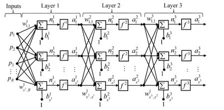
Figure 2: Multi-Layer Perceptron network
The output of one layer becomes the input to the next layer,

where M is the number of layers in the network and

The neurons in the first layer receive external inputs, which provides the starting point for Eq. (23), and the outputs of the neurons in the last layer are considered the network outputs,

For our case, the inputs to the ANN system are all the variables involved in the dynamic analysis of the laminated composite plate, which could include the material properties of the plies (,,,,,and), ply fiber-orientation angles (, i=1-NL)and ply thicknesses (ti , i=1-NL). We have only one output which is the fundamental natural frequency.
The standard back-propagation algorithm, presented by Hagan et al. [Hagan, Demuth and Beale (1996)], is used to adjust the different weights as well as the biases of the neural network. The back-propagation algorithm is a generalization of the Least Mean Square(LMS) algorithm. The LMS algorithm adjusts the weights and biases in order to minimize the mean square error performance index, where the error is the difference between the target output T and the network output a.

where P is the vector of network weights and biases.
3.1 Approximating function derivatives
Expressions for the first- and second-order derivatives were proposed in Deng et al. [Deng,Gu, Li et al. (2004); Breitung (1984)] considering only a single output for the ANN architecture. In the following two subsections, we present general expressions for the firstand second-order derivatives of any output of the ANN with respect to any input of any layer, not necessarily the input layer.
3.1.1 First-order output derivatives
First-order output derivatives are computed by applying a simple backward chaining partial differentiation rule. First, the derivatives of the NN outputs (outputs of the output layer M)with respect to the inputs of the same layer are calculated. Backward chaining is then employed to calculate the derivatives of the NN outputs with respect to its inputs. This is done as follows:
(i) For layer M:

where is the kthoutput of the output layer M.
(ii) For ahidden layer m (m = M - 2, …, 2, 1):

where, andis the number of neurons in layer m.
(iii) For the input layer:

where i is the input index, i=1:R , and l is the neuron index of the 1stlayer,, and piis the ithinput to the input layer.
3.1.2 Second-order output derivatives
The second-order partial derivatives of the network outputs, with respect to the inputs, are calculated using a backward chaining rule similar to that used for the first-order derivatives in previous section.
(i) For the neurons in layer M by substituting from Eq. (27):

(ii) For a hidden layer m (m = M - 2, …, 2, 1):

where

Substitute this expression into Eq. (31), we have

(iii) For the input layer:

Higher-order derivatives may be obtained in a similar fashion; however, the first- and second-order derivatives are the most commonly used for many practical applications.
4 Reliability models for the composite laminate
The first step in studying the variation of the fundamental frequency of a composite plate,, due to uncertainties in its geometric and material properties is to define a suitable and specific performance function. A composite plate is subjected to a harmonic load of frequency, which can take any value up to. In probabilistic design,is not a unique value, but is regarded as a random variable which has a certain distribution quantified by its mean and standard deviation. At the design point, the plate fundamental frequency, is equal to a certain specified value. To ensure a safe design, the value ofshould be lower than the plate natural frequency. Accordingly, a suitable performance function is defined as

whereare the plate eigenvalues, and X is a vector of basic random variables, given by

A failure surface or a limit state of interest can then be defined as g(X) = 0, with the probability of failure calculated as

whereis the joint probability density function (JPDF) for the n basic random variables, whereThe integration is performed over the failure region
There are several methods to calculate Pf. Here we shall use two types of analytical approximations that lead to two methods; the First-Order Reliability Method (FORM), and the Second-Order Reliability Method (SORM). Both methods will be used to predict the probability of failure and the Most Probable Point (MPP) of the system. A detailed description of both methods can be found in [Haldar and Mahadevan (2000); Shaker,Abdelrahman, Tawfik et al. (2008)] and will be summarized here.
In FORM and SORM, the partial derivatives of the performance function g(X) with respect to each random variable Xi, i=1, 2,…, n are required. These can be expressed as

Therefore, the partial derivatives of the fundamental eigenvaluewith respect to the problem basic variables Xiare required. These derivatives can be easily obtained from trained neural network as expressed in the previous section.
4.1 First-Order Reliability Method (FORM Method-2)
It is applicable to normal random variables. It first defines the reduced variables as

whereare random variables with zero mean and unit standard deviation. X coordinate system is referred to as the original coordinate system, whileis referred to as the transformed or reduced one; in which the transformed limit state equation is=0.The reliability (safety) index β is defined as the minimum distance from the origin of the axes in the reduced coordinate system to the limit state surface (failure surface, Fig. 3 (left)).It can be expressed as


Figure 3: (left) The reliability index, (right) FORM for nonlinear performance function
The minimum distance point on the limit state surface is called the checking point, design point, or Most Probable Point (MPP). It is denoted by the vectorin the original coordinate system and byin the reduced one.
For a nonlinear performance function, the gradient varies from point to point. The MPP has to be searched through the recursive formula given by Shaker et al. [Shaker,Abdelrahman, Tawfik et al. (2008)]

This formula can be geometrically interpreted from Fig. 3 (right). At each iteration point,the performance function is approximated by the tangent at this point, that is, the performance function is linearized withand
The algorithm is repeated until convergence, satisfying the following two criteria

where δ and ε are reasonably small numbers [Shaker, Abdelrahman, Tawfik et al. (2008)].
4.2 Second-Order Reliability Method (SORM)
A limit state function could be nonlinear either due to nonlinear relationship between random variables in the limit state equation or due to some variables being non-normal[Kaminski and Szafran (2015)]. A linear limit state in the original space becomes nonlinear when transformed to the standard normal space if any of the variables is non-normal.FORM methods use a first order Taylor series to approximate the limit state equation,ignoring its curvature, Fig. 4 (left). The SORM method improves the FORM results by including additional information about the curvature of the limit state equation using the second-order derivatives with respect to the basic random variables. Taylor series expansion of a general nonlinear function g(X) at the value (,, …,) is


Figure 4: Reliability Index for nonlinear performance functions (left), Rotation of coordinat(right)
A simple closed-form solution for the computation of the probability of failure using second-order approximation is derived using the theory of asymptotic approximations[Breitung (1984)] as

where β is the reliability index using FORM method, anddenotes the principal curvatures of the limit state at the minimum distance point. Φis the cumulative distribution function of a standard Gaussian distribution with zero mean and unit standard deviation.
Let Xidenotes a random variable in the original space, anddenotes the same random variable in the uncorrelated standard normal space. Thevariable is rotated to another variable, denoted bysuch that thevariable coincides with the vector α, the unit gradient vector of the limit state at the design point. This is shown in Fig. 4 (right) for two random variables.
The transformation from Y to Y′ is an orthogonal transformation

where R is the rotation matrix, computed as follow
(i) For two random variables:

where θ is the rotation angle as shown in Fig. 4 (right).
(ii) For more than two random variables, R is computed in two steps:
(a) Construct the matrix R0as follow:

where α1, α2, …, αnare the components of the unit gradient vector α at the design point.
(b) Apply a Gram-Schmidt orthogonalization procedure [Haldar and Mahadevan
(2000)] to R0whose rows are r01, r02, …, r0n, to get the matrix R whose rows are r1, r2, ..., rn. This procedure may be written as follows. The nthrow of R is simply rn= r0n, the other rows of R are computed in a backward order using the formula:


where d is the n×n second-derivative matrix of the limit state surface in the standard normal space evaluated at the design point andis the length of the gradient vector in the standard normal space.
In the rotated space the last variable Yn′ coincides with the β-vector computed in FORM;thus, the last column and last row in the A matrix and the last row in thevector are dropped to take this factor into account. The limit state can be rewritten in terms of a second-order approximation in the rotatedspace as

where A is now of the sizeFinally, the main curvatures κiare computed as the eigenvalues of the matrix A.
4.3 Monte Carlo Simulation (MCS) with Subset Simulation/Importance Sampling Method (SS/IS)
Monte Carlo simulation (MCS) techniques involve ‘sampling’ at ‘random’ to simulate artificially large number of experiments and to observe the results. The generation of random values for a random variable according to a specific distribution is the heart of Monte Carlo simulation. Solving the problem N times deterministically will give N sample points which can be used to calculate the entire sample statistics required: the frequency diagram, the PDF, the CDF, the corresponding parameters, and to evaluate the risk or reliability of an engineering system. The accuracy of the simulation increases as N increases. Plotting the estimated Pfand its corresponding variance show that these measures are reduced as the number of samples is increased and that a degree of stability is reached at a sufficiently high number of sample points. To overcome the inefficiency of the direct MCS, numerous variants of MCS (importance sampling, subset simulation) have been developed in the last two decades especially for the efficient solution of reliability problems where the calculation of small failure probabilities requires a very large sample size. Subset Simulation (SS) has been proposed in Au et al. [Au and Beck (2001); Song,Lu and Qiao (2009)]. It is a powerful tool, simple to implement and capable of solving a broad range of reliability problems. The basic idea of SS is to express the failure probability Pfas a product of larger conditional probabilities by introducing a decreasing sequence of intermediate failure events (subsets). The problem of simulating rare events in the original probability space is thus replaced by a sequence of simulations of more frequent events in the conditional probability spaces. Importance Sampling (IS) method is an efficient method for estimating conditional failure probability [Song, Lu and Qiao (2009)]. The choice of the intermediate failure events Fi(i =1, 2,…, m-1) plays a key role in the SS procedure.The more the simulation levels m is introduced, the larger the conditional failure probabilities, and smaller the sample size that estimations require. Then, the total sample sizeis large in the whole procedure. Conversely, if m is reduced, the conditional failure events become rare to obtain. Consequently, to have an accurate estimate of the conditional failure probabilities in each simulation level a larger sample size is required. It can be seen that the choice of the intermediate failure events is a compromise between Ni(the sample size required in each simulation level) and m (the number of simulation levels).
5 Numerical examples
MATLAB code was created to build a sample set, of size m, using the FEM model considering uncertainty of material properties, ply orientations and thicknesses. The sample set that includes the inputs (material properties, ply orientations and thicknesses)and the single target output (laminate fundamental natural frequency) is then used to train,validate and test the ANN, and obtain the corresponding weights and biases. This trained ANN is then used to calculate the safety index (β) and probability of failure (Pf) using FORM, SORM or MCS. Fig. 5 presents a schematic of the main files of the developed MATLAB code.
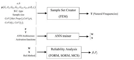
Figure 5: Schematic of the developed MATLAB code
In all the examples presented in this section a square SSSS laminate of dimensionscomposed of four plies, withis considered. Twenty-five (5×5) 9-noded elements are used in the FEM model, resulting in 121 nodes and 847 degrees of freedom. Unfortunately, there are no available established criteria for the selection of the MLP ANN architecture, and an educated guess based on the problem in hand is usually used to determine the best architecture [Lopes, Gomes and Awruch (2010)]. In all simulations, we used three layers of neurons, where the first layer has a number of neurons equal to the number of random variables, and the third layer has one neuron corresponding to the single output, whereas the middle layer has x neurons, where x is selected based on an educated guess in the range 0.6 n<x<1.4 n. Hence the architecture is: [n, x, 1]. Logsigmoid activation function was used in all the ANN layers except for the output layer where a linear activation function is used. All computations were done on a PC computer equipped with Intel Core i7, 3.4 GHz CPU, and 8 GB RAM, with a 64-bit WINDOWS10 operating system. The mean values and standard deviation of the basic random variables(mechanical properties in GPa, material density in Kg/m3, ply orientation angles in degree,and ply thickness in m) used in subsections 5.2 to 5.4 are shown in Tab. 1 [Singh, Yadav and Iyengar (2002); Shaker, Abdelrahman, Tawfik et al. (2008)]. The most used values ofis 0.97, so this value is used all over this study.

Table 1: Statistical distribution of the basic random variables
5.1 Code validation
First we present a validation for the FE model used to train the ANN by considering a square laminate with SSSS boundary condition and a/h=10 in order to compare the results with those given in Singh et al. [Singh, Yadav and Iyengar (2001); Shaker, Abdelrahman,Tawfik et al. (2008)]. The properties of the two materials used in Singh et al. [Singh, Yadav and Iyengar (2001)] are listed in Tab. 2. Tab. 3 and Tab. 4 show a comparison of the first five calculated non-dimensional natural frequencies, defined in Eq. (52), of a symmetric[0°/90°]slaminate of Material-1 and an anti-symmetric [0°/90°] laminate of Material-2. Two different mesh sizes are used and the results are compared with those presented in Singh et al. [Singh, Yadav and Iyengar (2001)]. It is clear from Tabs. 3 and 4 that a good agreement is obtained for the 2×2 mesh and an excellent agreement is obtained using the fine 5×5 mesh. The maximum difference is only 1.351% in the fifth non-dimensional natural frequency in Tab. 3. This small difference is believed to be due to the use of the full 3×3 integration rule in Singh et al. [Singh, Yadav and Iyengar (2001)]. The calculated values in Tab. 3 are identical to those reported in Shaker et al. [Shaker, Abdelrahman, Tawfik et al. (2008)].

Table 2: Material properties used in the validation [Singh, Yadav and Iyengar (2001)]
Table 3: Non-dimensional natural frequency for a SSSS [0°/90°]S square plate made of Material-1
[Singh, Yadav and Iyengar (2001)] Present Work 2×2 Present Work 5×5 % Δ5×5 11.77252 11.9187 11.7364 -0.306 21.83344 22.2978 21.8645 0.142 27.37726 28.0998 27.3512 -0.095 33.23205 34.4660 33.2477 0.047 37.43603 44.4042 37.9417 1.351
Table 4: Non-dimensional natural frequency for a SSSS [0°/90°]S square plate made of Material-2

Table 4: Non-dimensional natural frequency for a SSSS [0°/90°]S square plate made of Material-2
[Singh, Yadav and Iyengar (2001)] Present Work 2×2 Present Work 5×5 % Δ5×5 10.56565 10.8615 10.5589 -0.064 26.30276 27.9129 26.2667 -0.137 36.34791 38.4794 36.3033 -0.123 48.7006 48.9898 48.8484 0.303 55.14367 72.8828 55.2474 0.188
Now we present the validation for the ANN code by using a sample set of 1000 points with COV = 0.1 for material properties, density and ply orientation angles of a SSSS [0°/45°/-45°/90°] laminate, to train the ANN with [11,10,1] architecture. The ANN has been trained using 500 points, validated using 250 points and tested using 250 points. Training,validation and testing errors are plotted against the iteration number in Fig. 6. After 44 iterations, the training error reached 3×10⁻⁶, validation error reached 2.7×10⁻⁵, and the testing error reached 2×10⁻⁵. The mean, median and maximum error percentages of the test sample are as follows: mean=0.1183, median=0.0984, maximum=0.5119. Validation of the reliability analysis code (NNBSORM) is presented in subsection 5.3.
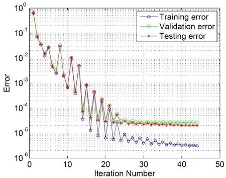
Figure 6: Training, validation and testing errors of the ANN. Case of SSSS [0°/45°/-45°/90°]laminate with [11,10,1] ANN architecture and 0.1 COV for material properties, density and ply orientation angles
5.2 Effect of considering Ply thickness uncertainty
One of the advantages of using the ANN to the reliability methods of analysis, such as FORM and SORM, is that it makes it possible to treat the ply thicknesses as random variables. This was impossible in previous attempt [Shaker, Abdelrahman, Tawfik et al.(2008)] where the reliability methods used the FEM model directly with the symbolic solver to differentiate the performance function with respect to all random variables. This is because it is impossible to explicitly express the derivatives of the D matrix (Eq. (15))with respect to the thicknesses of the plies tithat are not explicitly present in the components of D; rather the definitions of these components have terms that are function of z raised to some power as given in Eq. (16)
The effects of the uncertainty of the material properties, density, ply orientation angles and thicknesses on the coefficient of variance (COV) of the fundamental natural frequency of a [0°/90°]sand [0°/45°/-45°/90°] laminates are presented in Fig. 7 and Fig. 8 respectively. The mean values of the material properties are listed in Tab. 1. One thousand randomly generated points were used to generate each of these two figures. It can be seen from the figures that the uncertainty of the ply thicknesses has a more significant effect on the fundamental natural frequencies than that due to the uncertainty of ply orientation angles.In symmetric laminates (Fig. 7), the error in calculating COV (λ) by assuming deterministic ply angles is insignificant, but this error is significant if the ply thicknesses are assumed deterministic. In anti-symmetric laminates (Fig. 8), the error in calculating COV (λ) by assuming deterministic ply angles and thicknesses is significant and larger than that for the case of symmetric laminates. Hence it is concluded that, in addition to the uncertainty of the ply orientation angles, the uncertainty of the ply thicknesses should always be considered in the stochastic and reliability analysis of laminated composites.
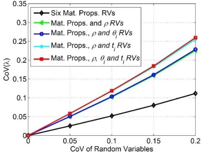
Figure 7: Variation of COV (λ) with simultaneous changes of the random variables for a SSSS [0o/90o]s square laminate
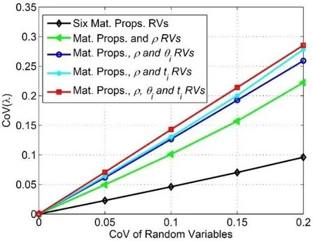
Figure 8: Variation of COV (λ) with simultaneous changes of the random variables for a SSSS [0 o/45 o/-45 o/90 o] square laminate
The first curve in Fig. 7 and Fig. 8 are almost identical to those presented in Singh et al.[Singh, Yadav and Iyengar (2001, 2002)], and the first three curves in these figures are almost identical to those presented in Shaker et al. [Shaker, Abdelrahman, Tawfik et al.(2008)]. This demonstrates once again the validity of our code. The upper two curves present for the first time the effect of ply thickness uncertainty on COV(λ) in addition to the uncertainty of the material properties and density of the plies, as well as the ply orientation angles in the uppermost curve.
5.3 Reliability analysis of a square composite laminate with deterministic ply thickness
In this example, the thicknesses of all plies are assumed deterministic in order to compare the results with published work [Shaker, Abdelrahman, Tawfik et al. (2008)]. The neural network architecture is [11,10,1] and 1000 points sample is used. Half of the sample points were used for training, quarter for validation, and quarter for testing. The mean error in λ obtained using the NN for this sample size was found to be 0.04%. The results using NNBR method are tabulated and compared with those obtained using SFEM [Shaker,Abdelrahman, Tawfik et al. (2008); Singh, Yadav and Iyengar (2002)] in Tab. 5 and Tab.6 for stacking sequence [0o/-45o/45o/90o]. The CPU time for SFEM with SORM [Shaker,Abdelrahman, Tawfik et al. (2008)] is reported as 2,484 sec which was very efficient compared to MCS that required 59,606 sec. The CPU time for the current model using NNBSORM is composed of the time (t1) required to generate the data points using FEM,the time (t2) required to train the ANN, and the time (t3) for calculating the MPP, β, and Pf.t1depends on the sample size, and t2depends on the ANN architecture used. For a big sample of 1000 points, t1= 1,348 sec, and for a [11, 10, 1] NN architecture, t2= 45 sec, and t3= 0.05 sec. Hence the total time is 1,393 sec, which is only about 56% the CPU time required for SFEM. As the number of plies increases, the saving in the CPU time gets bigger, making NNBSORM a much more efficient approach.
Table 5: MPP for SSSS [0°/45°/-45°/90°] square laminate with a/h = 10 for
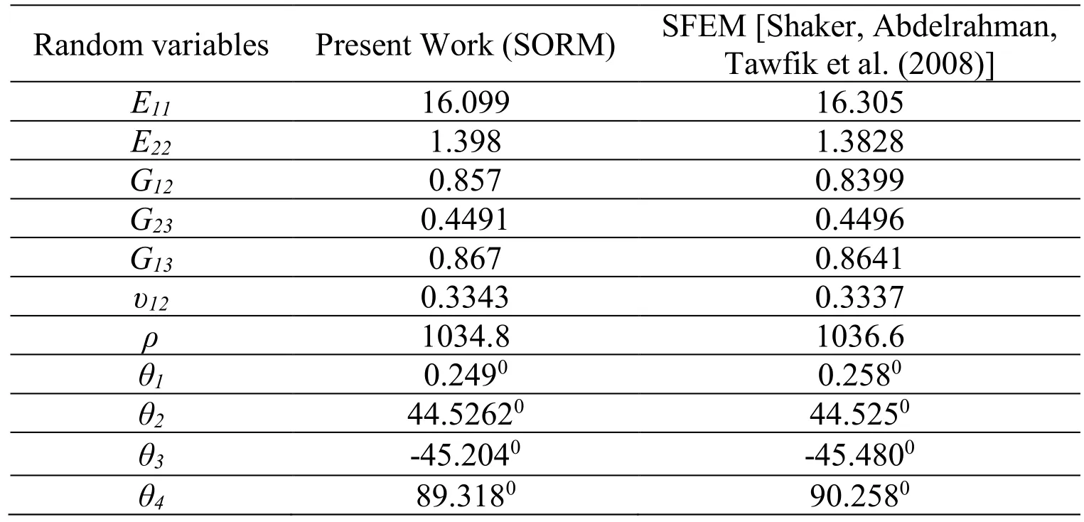
Table 5: MPP for SSSS [0°/45°/-45°/90°] square laminate with a/h = 10 for
Random variables Present Work (SORM) SFEM [Shaker, Abdelrahman,Tawfik et al. (2008)]E11 16.099 16.305 E22 1.398 1.3828 G12 0.857 0.8399 G23 0.4491 0.4496 G13 0.867 0.8641 υ12 0.3343 0.3337 ρ 1034.8 1036.6 θ1 0.2490 0.2580 θ2 44.52620 44.5250 θ3 -45.2040 -45.4800 θ4 89.3180 90.2580
Table 6: Comparison of the safety index and probability of failure for SSSS [0°/45°/-45°/90°]square laminate with a/h = 10 for
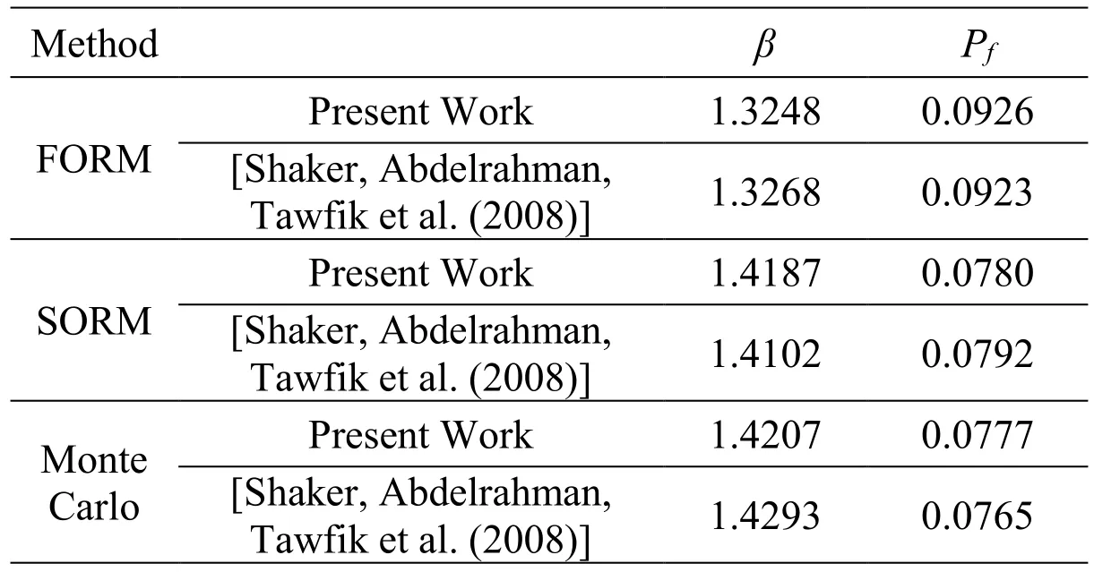
Table 6: Comparison of the safety index and probability of failure for SSSS [0°/45°/-45°/90°]square laminate with a/h = 10 for
Method β Pf FORM Present Work 1.3248 0.0926[Shaker, Abdelrahman,Tawfik et al. (2008)] 1.3268 0.0923 SORM Present Work 1.4187 0.0780[Shaker, Abdelrahman,Tawfik et al. (2008)] 1.4102 0.0792 Monte Carlo Present Work 1.4207 0.0777[Shaker, Abdelrahman,Tawfik et al. (2008)] 1.4293 0.0765
When the uncertainty in some variables is of a negligible effect on COV (λ), it is reasonable to ignore this uncertainty consider these variables deterministic. This will simplify the computation and makes it faster with almost no effect on the accuracy as was shown in the previous section for symmetric laminates. To verify this, the same laminate was analyzed considering the ply orientation angles (θ’s) as deterministic, and the results are shown in Tab. 7. By ignoring the uncertainty in the ply orientation angles, the ANN architecture is simpler, more efficient and requires a smaller sample size with almost no effect on the accuracy of the results.

Table 7: Comparison between random and deterministic stacking sequences with different NN architectures in an SSSS [0°/45°/-45°/90°] laminated composite plate
5.4 Reliability analysis of a square composite laminate with random Ply thickness
As mentioned in subsection 5.2 there has been no detailed investigation for the uncertainty in ply thicknesses on the laminates’ failure probability. In Section 5.2, it was shown that the uncertainty of ply thickness has a significant effect on the value of COV (λ). In this example, we analyze a [0o/45o/-45o/90o] SSSS composite plate with uncertain material properties (E11, E22, G12, G13, G23, υ12, ρ), and geometric properties (θi, ti). A sample of 1000 points was used for training the ANN, and the architecture used is [15, 20, 1]. The results using the proposed approach are tabulated in Tab. 8, showing more than 37% increase in the laminate probability of failure when ply thickness uncertainty is considered. This confirms the conclusion that was drawn previously that the uncertainty of the ply thicknesses should not be ignored in the reliability and optimization analyses of composite laminates.
Table 8: The probability of failure for SSSS [0°/45°/-45°/90°] square laminate with a/h=10 for

Table 8: The probability of failure for SSSS [0°/45°/-45°/90°] square laminate with a/h=10 for
Present Work Thicknesses of all plies are deterministic Thicknesses of all plies are random FORM 0.0926 0.115 SORM 0.0780 0.109 Monte Carlo 0.0777 0.107
6 Summary and conclusion
This paper presents reliability analysis of freely-vibrating fiber-reinforced laminated composite plates taking into account the uncertainty of its material and geometric properties. The analysis was performed using a new method that combines the Second Order Reliability Method (SORM) with a trained artificial neural network (ANN). The use of ANN improves the efficiency of the simulations because the need for using symbolic solvers to differentiate the performance function with respect to the random variables was totally eliminated. Moreover, the utilization of the ANN allowed for the consideration of ply thicknesses uncertainty. The effect of ply thicknesses randomness, which was not considered in previous published works, was found to be pronounced and should not be ignored if an accurate reliability analyses of composite structures are to be done.
Explicit expressions for the first and second derivatives of the ANN output (laminate fundamental natural frequency) with respect to any of the inputs (ply material and geometrical properties) are presented. The implementation of these expressions made the whole process to be numeric without any symbolic calculations. The finite element model is just used to train the ANN.
Using the proposed NNBSORM, a significant saving in the computational time without loss in accuracy was achieved. The probability of failure Pfwas calculated using the proposed methodology. The comparison between the results obtained and those given in published works has shown that more than 40% reduction in the computation time for the case of a laminate composed of four plies was achieved. The efficiency of the simulations is higher than that of the SFEM especially for problems containing a large number of random variables, as in the case of laminates with large number of plies. Future work will focus on utilizing the Radial Basis Functions ANN architecture in the formulation of the NNBSORM.
Acknowledgment:The first and third authors acknowledge the support of Cairo University, Egypt. The second author acknowledges the support of California State University, Northridge.
Appendix A. Expressions of

where the lamina invariants are:

and

Apalak, M. K.; Yildirim, M.; Ekici, R.(2008): Layer optimisation for maximum fundamental frequency of laminated composite plates for different edge conditions.Composites Science and Technology, vol. 68, no. 2, pp. 537-550.
Au, S. K.; Beck, J. L.(2001): Estimation of small failure probabilities in high dimensions by subset simulation. Probabilistic Engineering Mechanics, vol. 16, no. 4, pp. 263-277.
Breitung, K.(1984): Asymptotic approximations for multinormal integrals. ASCE Journal of Engineering Mechanics, vol. 110, pp. 357-366.
Chapman O. J.; Crossland, A. D.(1995): Neural networks in probabilistic structural mechanics. In C. (Raj) Sundararajan, editor, Probabilistic Structural Mechanics Handbook,pp. 317-330. Chapman & Hall, New York, USA.
Chiachio, M.; Chiachio, J.; Rus, G.(2012): Reliability in composites-a selective review and survey of current development. Composites: Part B, vol. 43, pp. 902-913.
Deng, J.; Gu, D.; Li, X.; Yue, Z.(2004): Structural reliability analysis for implicit performance functions using artificial neural network. Structural Safety, vol. 26, pp. 123- 139.
Gomes, H.; Awruch, A. M.(2004): Comparison of response surface and neural network with other methods for structural reliability analysis. Structural Safety, vol. 26, no. 1, pp.49- 67.
Gosling, P. D.; Faimun, Polit, O.(2014): A high-fidelity first-order reliability analysis for shear deformable laminated composite plates. Composite Structures, vol. 115, pp. 12-28.
Hagan, M. T.; Demuth, H. B.; Beale, M. H.; De Jesus, O.(2014): Neural Network Design. PWS, Oklahoma, USA.
Haldar, A.; Mahadevan, S.(2000): Probability, reliability and statistical methods in engineering design. Wiley, New York, USA.
Hosni Elhewy, A.; Mesbahi, E.; Pu, Y.(2006): Reliability analysis of structures using neural network method. Probabilistic Engineering Mechanics, vol. 21, no. 1, pp. 44-53.
Hurtado, J. E.(2002): Analysis of one-dimensional stochastic finite elements using neural networks. Probabilistic Engineering Mechanics, vol. 17, pp. 35-44.
Hurtado, J. E.(2004): Structural reliability. statistical learning perspectives. Springer,Heidelberg Springer-Verlag, Berlin Heidelberg, Germany.
Hurtado, J. E.; Alvarez, D. A.(2001): Neural-network-based reliability analysis: A comparative study. Computer Methods in Applied Mechanics and Engineering, vol. 191,no. 1-2, pp. 113-132.
Kaminski, M.; Szafran, J.(2015): Least squares stochastic finite element method in structural stability analysis of steel skeletal structures. Computer Modeling in Engineering& Sciences, vol. 107, no. 1, pp. 27-57.
Lopes, P. A. M.; Gomes, H. M.; Awruch, A. M.(2010): Reliability analysis of laminated composite structures using finite elements and neural networks. Composite Structures, vol.92, no. 7, pp. 1603-1613.
Nazari, F.; Abolbashari, M. H.; Hosseini, S. M.(2015): Three dimensional natural frequency analysis of sandwich plates with functionally graded core using Hybrid Meshless Local Petrov-Galerkin method and artificial neural network. Computer Modeling in Engineering and Sciences, vol. 105, no. 4, pp. 271-299.
Oh, D. H.; Librescu, L.(1997): Free vibration and reliability of composite cantilevers featuring uncertain properties. Reliability Engineering & System Safety, vol. 56, pp. 265-272.
Papadrakakis, M.; Papadopoulos, V.; Lagaros, N. D.(1996): Structural reliability analysis of elasticplastic structures using neural networks and Monte Carlo simulation.Computer Methods in Applied Mechanics and Engineering, vol. 136, pp. 145-163.
Papadrakakis, M.; Lagaros, N. D.; Tsompanakis, Y.(1998): Structural optimization using evolution strategies and neural networks. Computer Methods in Applied Mechanics and Engineering, vol. 156, pp. 309-333.
Reddy, J. N.; Robbins, D. H.(1994): Theories and computational models for composite laminates. Applied Mechanics Reviews, vol. 47, no. 6, pp. 147-169.
Salim, S. (1995): Analysis of Composite Plates with Randomness in Material Properties(Ph.D. Thesis). Department of Aerospace Engineering, IIT Kanpur, India.
Salim, S.; Yadav, D.; Iyengar, N. G. R.(1992): Deflection of composite plates with random material characteristics. Proceedings of Symposium on Recent Advances in Aerospace Science and Engineering Conference, vol. 1, Bangalore, New Delhi, pp. 236-239.
Salim, S.; Yadav, D.; Iyengar, N. G. R.(1993): Analysis of composite plates with random material characteristics. Mechanics Research Communications, vol. 20, no. 5, pp. 405-414.
Santos, S. R.; Matioli, L. C.; Beck A. T.(2012): New optimization algorithms for structural reliability analysis. Computer Modeling in Engineering and Sciences, vol. 83,no. 1, pp. 23-55.
Schueremans, L.; Gemert, D. V.(2005): Benefits of splines and neural networks in simulation based structural reliability analysis. Structural Safety, vol. 27, pp. 246-261.
Shaker, A.; Abdelrahman, W. G.; Tawfik, M.; Sadek, E.(2008): Stochastic finite element analysis of the free vibration of laminated composite plates. Computational Mechanics, vol. 41, pp. 493-501.
Shankara, C. A.; Iyengar N. G. R.(1996): A Coelement for the free vibration analysis of laminated composite plates. Journal of Sound and Vibration, vol. 191, no. 5, pp. 721-738.
Singh, B. N.; Yadav, D.; Iyengar N. G. R.(2001): Natural frequencies of composite plates with random material properties using higher order shear deformation theory.International Journal of Mechanical Sciences, vol. 43, pp. 2193-2214.
Singh, B. N.; Yadav D.; Iyengar N. G. R.(2002): A Coelement for free vibration of composite plates with uncertain material properties. Advanced Composite Materials, vol.11, no. 4, pp. 331-350.
Song, S.; Lu, Z.; Qiao, H.(2009): Subset simulation for structural reliability sensitivity analysis. Reliability Engineering & System Safety, vol. 94, no. 2, pp. 658-665.
Zhang, S.; Zhang, L.; Wang, Y.; Tao, J.; Chen, X.(2016): Effect of ply level thickness uncertainty on reliability of laminated composite panels, Journal of Reinforced Plastics and Composites, vol. 35, no. 19, 1387-1400.
 Computer Modeling In Engineering&Sciences2018年4期
- Computer Modeling In Engineering&Sciences的其它文章
- Loose Gangues Backfill Body’s Acoustic Emissions Rules During Compaction Test: Based on Solid Backfill Mining
- Three-Variable Shifted Jacobi Polynomials Approach for Numerically Solving Three-Dimensional Multi-Term Fractional-Order PDEs with Variable Coefficients
- Simulation of Stochastic Ice Force Process of Vertical Offshore Structure Based on Spectral Model
- Grey Wolf Optimizer to Real Power Dispatch with Non-Linear Constraints
- Statistical Multiscale Analysis of Transient Conduction and Radiation Heat Transfer Problem in Random Inhomogeneous Porous Materials
