Reconstructing the size of individual trees using log data from cut-to-length harvesters in Pinus radiata plantations:a case study in NSW,Australia
Kuan Lu·Huiquan Bi·Duncan Watt·Martin Strandgard·Yun Li
Introduction
Originating from and developed in the Scandinavian countries since the 1970s(see Hellstr?m et al.2009;Nordfjell et al.2010),cut-to-length(CTL)harvesters have been increasingly adopted and widely utilised in forest harvesting operations worldwide.Besides northern and other European countries,the utilisation of CTL technology has greatly improved the productivity of harvesting in many other countries around the world(e.g.,Huyler and LeDoux 1999;Murphy 2003;Gerasimov et al.2012,2013;Strandgard et al.2013;Olivera et al.2016;Williams and Ackerman 2016),particularly in plantation forestry where trees are usually harvested before they become too large to be handled by machines and tree size is more uniform.The past 40 years has seen great technological advances in the mechanical design of harvesters and in the harvester head measurement and optimization systems as reviewed by Heinimann(2007),Nordfjell et al.(2010),Uusitalo(2010)and Malinen et al.(2016).However,the basic concept has remained the same among CTL harvesters of different makes,models and ages(Heinimann 2001;Uusitalo 2010;Spinelli et al.2011;Malinen et al.2016).All have a cutting head attachment that is capable of felling,delimbing,measuring and processing stems.A typical harvester head consists of(1)a chain saw to fell a tree at its base and cut the stem to length;(2)one or two pairs of curved delimbing knives that reach around the stem to remove branches;(3)two,three or four feed rollers to grasp the tree and to force the cut stem through the delimbing knives;(4)diameter sensors to measure the diameter overbark(DOB)of the cut stem;and(5)a measuring wheel to measure log length as the stem is fed through the head.Depending on the make and model of harvester,the diameter sensors are connected to either the top or the bottom delimbing knives or to the feeding roller arms,and diameter measurement depends on how wide the knives or feeding arms open(Nieuwenhuis and Dooley 2006;Miettinen et al.2010).The diameter and length measurements are recorded by an onboard computer every time a log is cut.Based on the measurements,the computer system optimizes log cutting according to the pre-programmed speci fications of log length,end diameters,quality and their price list to ensure the highest values are recovered from the trees being harvested.
Despite the sophisticated measurement and optimisation systems,the current generation of harvester heads are not able to measure stump height and diameter(i.e.,large end diameter of the butt log)as the chain saw makes the first cut to fell a tree.They are also unable to measure the length from the last cut(i.e.,small end of the top log)to the tip of the tree as this section does not pass through the harvester head.So it is impossible to obtain any data on total tree height as the trees are felled and bucked.Noncontact laser scanning methods to measure a tree stem before felling and during the cut-to-length process still remain as an experimental concept for harvester heads at this stage(?hman et al.2008;Miettinen et al.2010;Vanclay 2011;Kong et al.2015).The common and standard practice has been to assume an average stump height for all trees based on empirical data from post-harvesting surveys or to use a speci fied stump height of 10 cm as documented in Stan-ForD 2010,the Standard for Forest Machine Data and Communication that has been developed,coordinated and maintained by Skogforsk(the Forestry Research Institute of Sweden)since its initiation in 1988(Arlinger et al.2012).Even so,it is impossible to measure stump diameter right at the height of the first cut as the delimbing knives or the feed rollers for measuring diameter are mounted at a certain height above the chain saw.This height differs among the makes and models of harvesters.For example,the John Deere H290 harvester head measures DOB using the bottom delimbing knives that are mounted 20 cm above the saw,while the John Deere H480 uses the top knives that are 80 cm above the saw.In comparison,the Log Max 6000 measures DOB through its feed rollers 130 cm above the saw(J.Rombouts,pers.comm.).In such cases,the height of the first DOB measurement may vary from a minimum of 20 cm to a maximum of 130 cm above the stump,i.e.,greater than the de fined breast height of 1.3 m above ground level when stump height is included.
Many harvester heads currently in operation use the first DOB measurement to derive the overbark diameter at breast height(DBHOB,de fined as 1.3 m above ground level in Australia).So DBHOB is normally an extrapolated diameter since the harvester head usually measures the first diameter some decimeters below 120 cm above the stump as documented in StanForD 2010.The first DOB measurement is also used in deriving the stump diameter,i.e.,the large end diameter of the butt log through extrapolation.When DBHOB is a measured value,a height above stump height for taking the measurement must be speci fied(e.g.120 cm in Finland and Sweden,and 110 cm in Norway)based on an assumed average stump height or on the mean stump height from postharvesting surveys(Holopainen et al.2010).The measured DBHOB and other diameter measurements taken at 10-cm intervals starting at the height of the first diameter measurement can be stored together in individual stem files(.stm)in the onboard computer for deriving stem pro files through spline-based smoothing curves(e.g.,Nummi and M?tt?nen 2004;Koskela et al.2006;Barth and Holmgren 2013).In the most advanced harvester heads,diameter recordings can be obtained at much smaller(about 1 cm)intervals and stored in stem files.The data are filtered to remove noises due to branches,jitters,shakes and other causes before they are used to derive stem pro files from which DBHOB can be obtained(T.Pukkala,pers.comm.).
With their widespread utilization,CTL harvesters have become a major source of ‘big data’for forest management as they constantly capture and provide a daily flow of detailed information on log production and assortment as well as detailed diameter measurements of tree stems(Sellén 2016).Harvester data have been used in combination with conventional inventory data to develop harvester-based forest inventory systems(Stendahl and Dahlin 2002;Murphy et al.2006;Holopainen et al.2010)and with remote sensing imagery and LiDAR data to predict attributes of individual trees,stands and forests(Rasinm?ki and Melkas 2005;Holmgren et al.2012;S?derberg 2015),product recovery(Peuhkurinen et al.2008;Barth and Holmgren 2013;Barth et al.2015),and wood properties(M?ller et al.2003).Such combined use of harvester data creates a representation of the entire forest area in great detail,allowing forest managers to see what trees are standing where and to predict what volume or value of a certain product or a product mix the forest can yield.Operationally,harvester data have mainly been used to improve value recovery and production planning,to monitor product length mix from areas being harvested in thinning and clear-fell operations,and to reduce production risks through fewer rejects.
Harvester data afford the calculation of the total length between the stump and the last cut but not the total height of individual trees.Apart from log length,diameters and limited quality and defect information,other tree and stand attributes pertaining to the harvested forest no longer exist.As well-recognised and demonstrated in the literature(e.g.,Kiljunen 2002;Maltamo et al.2010;S?derberg 2015;Siipilehto et al.2016),tree and stand reconstructions of the harvested forest are a necessary first step to provide the essential link for the most effective use of harvester data.This first step involves the estimation of DBHOB and total height of individual trees using harvester data.The need for estimating DBHOB arises when the harvester data set at hand or the extracted database from it contains only the length,volume and small end diameter of individual logs cut from each stem and stem- files are not available due to time lapse,operating and processing issues and system de ficiencies.DBHOB may also not be recorded in the stem files as it is an optional variable in the StanForD standard.Total tree height can be calculated through the estimation of the length of the unprocessed top section of individual trees(Kiljunen 2002;Maltamo et al.2010).
Pinus radiata D.Don is a major softwood plantation species in the Southern Hemisphere(Lewis et al.1993;Mead 2013),and it covers a total area of approximately 772,100 ha in Australia(Downham and Gavran 2017).About one-third of this plantation resource is in the State of New South Wales(NSW).Following an initial experience of using imported machines from Sweden for thinning in the early 1980s,CTL harvesters were introduced into Australia for final harvesting in the early 1990s(Priddle 2005).Over the last 20 years,harvesting companies and/or contractors across Australia have gradually adopted the CTL technology,but with varying degrees of familiarity,sophistication and consistency in capturing,managing and using harvester data for forest management and planning.Monitoring and summarizing harvesting production and log yields have remained the main use of harvester data in many forestry companies.However,researchers have used harvester data to estimate harvester productivity and,in combination with terrestrial laser scanning,to determine tree value and log yields in P.radiata plantations(Strandgard et al.2013;Murphy et al.2010).A research project is currently being carried out to combine harvester data with airborne LIDAR to estimate stand volume and log yield of a plantation,for which trees and stands needs to be reconstructed from harvester data.To facilitate such reconstructions,this study aims to develop(1)a system of equations for estimating DBHOB of trees from diameter overbark(DOB)measured by a harvester head at any height up to 3 m above ground level and(2)an equation to predict the total height of harvested stems from harvester data in the P.radiata plantations of NSW,Australia.
Materials and methods
Data
For accomplishing the objectives,it would be ideal if the total tree height and the stump height of harvested stems were available in addition to the number of logs,their lengths and end diameters recorded by harvesters.However,apart from log length and diameter,other tree attributes pertaining to the harvested stems could not be measured by harvester heads,posing a dif ficulty for the intended analysis.To overcome this dif ficulty,three data sets were used in combination to construct a simulated data set that not only included stump height and total tree height but also mimicked the cutting patterns of harvesters in operational harvesting.The first was a compilation of taper data with DBHOB,total tree height and sectional diameter measurements of a large number of sample trees.The taper data were used to(1)derive a set of relationships for converting diameter at the first point of measurement at a range of speci fied heights above ground level to DBHOB and(2)construct stem pro files of individual trees that were cut to length in the simulated log cutting.The second data set contained stump heights from postharvesting surveys,which were used to specify a stump height in the cutting simulation.The third was a harvester data set with records of log length,volume and small end diameter of all logs cut from each stem.The harvester data were used to derive patterns for the simulated cutting of the constructed stem pro files.The combined use of the three data sets and the simulated CTL data ful filled the data requirement of the study.To aid readers’understanding of the coming sections of this paper,the entire data processing and analytical work flow was summarized and outlined in a flowchart(Fig.1).
Taper data
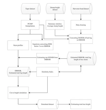
Fig.1 A flowchart outlining the entire data processing and analytical work flow.The section numbers in the boxes indicate where the steps were described in the text
The taper data included 3251 trees sampled from P.radiata stands across NSW over a period of thirty years.The data were previously used to develop taper and height–diameter functions(Bi and Long 2001;Bi et al.2012),and conversion factors for DBHOB measured at different breast height(Zhang et al.2015).As described by Bi and Long(2001),the sample trees had an age range between 10 and 47 years,and they were taken from both thinned and unthinned stands.Taper measurements were relatively consistent.The lowest measurements of both overbark and underbark diameters were taken at between 0.1 m to 0.3 m above ground,then another measurement was usually taken at 0.7 m before reaching the de fined breast height of 1.3 m.Measurement intervals above breast height varied between 1.5 to 3 m depending on the height of the sample trees.The number of measurement points over the lower stem below 5 m varied mostly from 4 to 6 among the 3251 sample trees.For the purpose of this study,86 trees that had underbark but not overbark taper measurements were excluded,leaving a total of 3165 trees in the taper data set(Fig.2).
Stump height data
The data came from postharvesting surveys of stump height conducted as part of routine residue and waste assessment in clearfall operations using CTL harvesters between 2012 and 2015 in P.radiata plantations of the Snowy Region of Forestry Corporation of NSW(FCNSW).The region manages about 120,000 ha of P.radiata plantations on the south-west slopes of NSW and supplies customers 1.35 million m3of sawlogs and 0.86 million m3of pulpwood annually through long-term wood supply agreements according to the FCNSW’s 2016 forest management plan.The data contained height measurement of 4676 stumps from 125 transects established over 31 postharvesting sites(Fig.3).Stump height was measured from ground level on the high side of the stump to a point level with the top of the stump,but stump diameter was not measured in the surveys.The length of transects varied from 50 to 400 m,but the majority of transects had a length of 200 m.
Harvester data
A sample of harvester data was also provided by the Snowy Region of FCNSW for the purpose of this study.The data contained a total of 16,243 stems/trees that were harvested and processed by CTL harvesters in routine second thinning operations in 22-year-old P.radiata plantations in seven compartments of Bungongo State Forest in the Tumut management area in 2013.Second thinning data were used as the trees cover a large range of tree height and DBHOB values.Each stem was cut into several logs numbered sequentially from the butt to the end near the tip and their length,overbark volume and small end diameter overbark(SEDOB)were recorded.But large end diameter overbark(LEDOB)of the butt log(i.e.,stump diameter)was not available.A total of 65,287 logs were recorded in the sample data set.The cutting patterns were largely driven by the small log speci fications for the domestic market,the sawlog speci fications for Carter Holt Harvey Woodproducts Australia,and the pulpwood speci fications for Visy Industries.Both companies are major long-term customers of the Snowy Region of FCNSW.Stump height,DBHOB and total tree height were not available from the harvester data.Individual stem files for the stems were not recorded or not available due to the lapse of time.

Fig.2 Scatter plot and frequency distributions of DBHOB and total tree height of the 3165 trees in the taper dataset.The lower and upper curves represent the 0.005th and the 0.995th nonlinear conditional quantiles(see Eq.11 and text in Sect.4.2,)
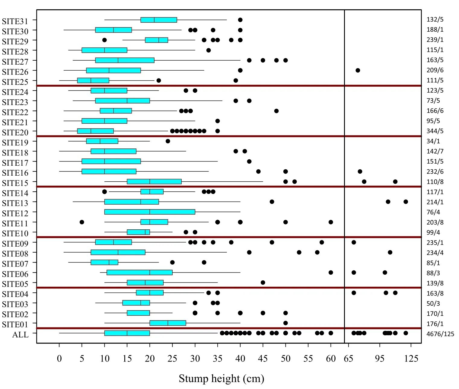
Fig.3 Boxplots of stump height for the 31 survey sites and for all sites combined as indicated by the labels on the left hand side.Numbers before and after the forward slash on the right hand side indicate the number of stumps measured and the number of transects surveyed respectively.The vertical line between stump height 60 and 65 cm was drawn to show the graph in two different scales to avoid the majority of the data points being obscured by a small number of extreme values
As is often the case with harvester data,a number of erroneous and illogical records were detected following a careful data screening and exploratory data analysis.For the intended use of the harvester data in this study,i.e.,to derive patterns for the simulated log cutting of the stem pro files constructed from taper data,a two-stage data screening process was carried out.In the first stage,frequency distributions and descriptive statistics of the number of logs cut from individual stems and that of the total log length were examined.A total of 172 stems had 8 or more logs,including the extreme cases of 17,18 and 42 logs cut from a single stem as recorded in the harvester data(Fig.4).Some of these trees may have had multiple leaders and/or short defective sections.There were also five trees with a total log length less than 3 m,shorter than the shortest speci fied length for a pulp log.These 177 trees were removed from the data set.In the second stage,the sequentially numbered logs from each stem were examined in relation to their product speci fications and in terms of their pattern of change in SEDOB over the accumulative log length,i.e.,height above stump.Stems with more than half of its logs not assigned to any product category in the harvester data were considered to be dubious or deformed trees.Trees with the smallest SEDOB greater than 20 cm,i.e.,the upper limit of the speci fied SEDOB(8–20 cm)for small logs,might be only partially processed by the harvester head due to breakage or other damage to the upper stem.A number of stems had the same values of recorded SEDOB for two or more logs that were cut at least 3 m apart,which might be caused by a bulge,a branch knot or simply recording errors of the harvester head.By contrast,there were other stems whose log SEDOB decreased far too rapidly when plotted against the cumulative log length.These cases might be associated with double or multiple leader trees that could not be marked by the harvester head.Considering the intended use of the harvester data in this study,these stems,2422 in total,were also removed from the data set,leaving a final data set containing a total of 13,644 stems and 55,222 logs for the log cutting simulation.The relatively large proportion of defective stems was likely to re flect that the data were from a second thinning operation which has the removal of defective stems as a primary objective.
Converting DOB at any height below 3 m to DBHOB
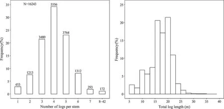
Fig.4 Frequency distribution of the number of logs cut from a single stem(left)and that of their total log length(right).N indicates the total number of stems contained in the harvester data.The number on top of each bar indicates the number of stems in that category
Because the height of the first DOB measurement taken by a harvester head during tree harvest can vary from a minimum of 20 cm to a maximum of 130 cm above the stump,which can vary in height from less than 10 cm to 50 cm or more above ground level(Fig.3),it would be ideal to be able to derive an estimate of DBHOB from DOB measured at any height within a de fined range above ground level.Considering the makes,models and ages of all harvesters currently in operation,a range between 0 and 3 m above ground level was adopted to accommodate all possible heights of the first DOB measurement.Within this range,30 heights from 0.05 to 2.95 m with an even interval of 0.1 m were selected to develop height-speci fic equations to convert DOB to DBHOB.However,actual field measurements of DOB at the 30 speci fied heights above ground level were not available from any sources of empirical data.To overcome this dif ficulty,the taper data were used to obtain numerically interpolated values of DOB at the 30 speci fied heights for each of the 3165 trees in the taper data set using piecewise cubic hermite interpolating polynomials(PCHIP)implemented in MATLAB(R2015b).This particular interpolation method was adopted because it was proven to be the most accurate after a detailed evaluation and comparison with three other methods including the polynomial interpolation of Lagrange,that of Newton,and cubic spline interpolation(Zhang et al.2015).An example of DBHOB plotted against interpolated values of DOB at 8 of the 30 speci fied heights is shown in Fig.5.
To convert DOB measured at any of the 30 speci fied heights to DBHOB,a system of 30 equations was speci fied as follows:

where ln stands for natural logarithm,DBHOB is in cm,DOBh1...DOBh30denote DOB in cm at the 30 speci fied heights(h1…h(huán)30)above ground level,ranging from 0.05 to 2.95 m at an even interval of 0.1 m, αh1...αh30,and βh1...βh30are the parameters to be estimated,and ε1… ε30are the corresponding error items that were assumed to jointly follow a multivariate normal(MVN)distribution with a zero mean vector and a positive de finite covariance matrix.The system of 30 equations was first estimated by the ordinary least squares(OLS)estimator in the PROC MODEL procedure of SAS 9.4 without considering the inherent cross-equational error correlations.To take into account the inherent correlations,the system was also estimated by using the seemingly unrelated regression(SUR)estimator of Zellner(1962)to achieve greater ef ficiency in parameter estimation(Srivastava and Giles 1987).Mean squared error(MSE)and R2values were computed for individual equations.The use of logarithmic regression in the system of equations would certainly incur bias in the estimation of DBHOB when the predicted values were back-transformed from logarithm.The existence of such an inherent bias in logarithmic regression has been well recognised(e.g.,Baskerville 1972;Flewelling and Pienaar 1981;Snowdon 1991).To correct for such bias,Snowdon’s(1991)bias correction factor was calculated for each of the 30 system equations following parameter estimation so that DOB measured at any of the 30 speci fied heights could be converted to DBHOB as follows:

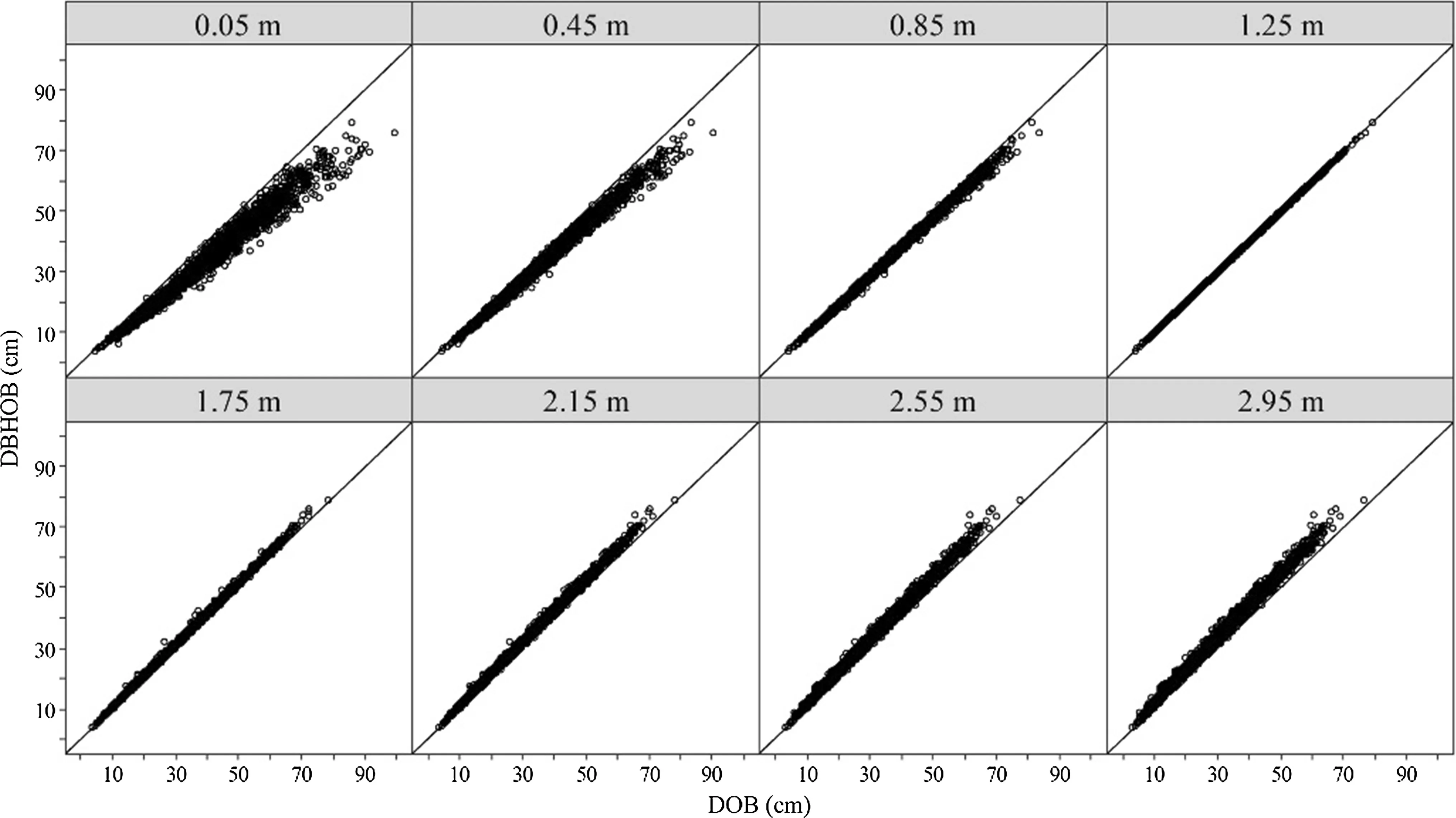
Fig.5 A multipanel display of DBHOB plotted against diameter overbark(DOB)at 8 of the 30 speci fied heights above ground level as marked in the top strip of each panel for the 3165 trees in the taper dataset.The diagonal line in each panel is the line of unity
Although the 30 speci fied heights covered a complete height range of the first DOB measurement by any harvester head regardless of its make,model and age,in practice the first DOB may not be taken exactly at any one of speci fied heights.In such cases,simple linear or the nearest interpolation of the estimated parameters and bias correction factors of the system equations in model(1)would be the two most obvious options for obtaining a unique set of parameters at any given height below 3 m above ground level for the conversion of DOB to DBHOB.To evaluate the accuracy of these two approaches and of the system of equations in converting DOB to DBHOB at any height below 3 m,another data set was generated firstly by randomly selecting a height within each of the 29 intervals in between the 30 speci fied heights.The selected heights were based on random numbers generated from the uniform distribution but did not include the 30 speci fied heights at which the data were already used for parameter estimation.For these 29 randomly selected heights,the conversion parameters and bias correction factors were then derived from those for the 30 system equations in model(1)using the two interpolation methods:simple linear interpolation and the nearest interpolation,i.e.,taking the estimated parameters and the calculated bias correction factor of the nearest speci fied height.In addition,29 interpolated values of DOB were obtained also using PCHIP for each of the 3165 trees contained in the taper data set.These DOB values were finally converted to DBHOB using the the conversion parameters and bias correction factors obtained through the two interpolation methods.Using the observed and converted values of DBHOB,we calculated the mean error of prediction(MEP),the mean absolute error of prediction(MAEP),the mean squared error of prediction(MSEP),and the prediction coef ficient of determinationfor each of the randomly selected height as follows:
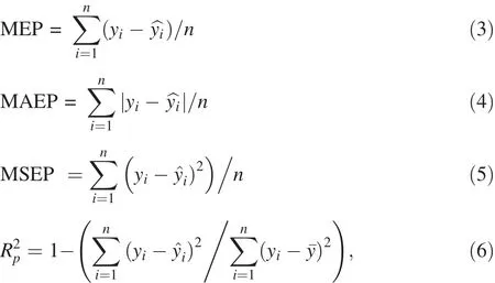
where yirepresents the observed DBHOB of the ith tree in cm,stands for the value of DBHOB converted from DOB at the selected height for the same tree,y is the mean observed DBHOB,and n isthetotalnumberof observations,equal to 3165 trees in this case.As reviewed by Huang et al.(2003),the four benchmarking statistics have been commonly used in evaluating the predictive performance of forest models as they assess the size,direction and dispersion of the prediction error.In particular,the MSEP is the measure of prediction accuracy commonly used in the statistical literature since it incorporates both the variance of prediction error and the bias of prediction(Wackerly et al.1996).Analogous to the coefficient of determination R2,is essentially the model ef ficiency coef ficient originally proposed by Nash and Sutcliffe(1970).But unlike R2,which ranges from 0 to 1,can range from-∞to 1.Anof 1 corresponds to a perfect match of the predicted to the observed values,while anof 0 indicates that the model predictions are as accurate as the mean of the observed values.When the observed mean is a better predictor than the model,the value ofis less than 0,as the residual variance is larger than the variance of the observed data.
Estimating total tree height from harvester data
Because the stump height and the top section of a tree are not measured by the harvester head,it is impossible to develop equations for predicting total tree height using the harvester data per se.The harvester data must be used with the taper data to generate a data set that contained stump height(0.15 m,i.e.,the average stump height over all sites in Fig.3),the number of logs,their length,LEDOB and SEDOB values,and more importantly,the length of the top section of every tree.Such a data set was generated through simulated log cutting of the complete stem pro files of trees from ground to tip constructed from their taper data.The cutting patterns used in the CTL simulations were extracted from the harvester data for individual trees in the taper data set.The simulated data set would then enable the development of equations for predicting total tree height from harvester data.
Cut-to-length(CTL)simulations
During harvesting operations in P.radiata plantations,trees with DBHOB less than 10 cm are not harvested because they are unmerchantable.Thus,66 trees of such sizes in the taper data set were not included in the logcutting simulation,leaving 3099 trees in the data set.For each tree in this data set,the simulation went through the following steps:(1)estimating its potential total log length;(2)selecting the stem that was most similar in DBHOB and total log length from among the 13,644 stems in the harvester data;(3)adjusting the cutting pattern of the most similar stem before using it to locate the sequential crosscut points on its stem pro file that was interpolated from taper measurements;(4)calculating the DOB at each cutting point using the interpolated stem pro file;(5)exporting the values of stump height,log number,length,LEDOB and SEDOB,and the length between the last cutting point to the tip of the tree to a holding data set for further analysis(Fig.6).
To complete step 1,a nonlinear equation was derived first to predict the SEDOB of the top log(i.e.,the smallest SEDOB of a stem)from DBHOB using the harvester data.After some exploratory analysis and comparisons of several model forms,the following equation form was adopted:

where SEDOBTLis the SEDOB of the top log in cm,a and b are parameters.Equation(7)was fitted using median regression instead of the least squares method because of the extent of the spread of the 13,644 data points and at the same time because of the desire to avoid some outliers exerting an undue in fluence on the parameter estimates.The R package for quantile regression,quantreg(Koenker 2015,2016,2017),was used to estimate the two parameters for the 0.50th nonlinear conditional quantile.Because the harvester data did not contain DBHOB for the stems,the SEDOB of the first section,either a butt log or a much shorter waste or off-cut section between the stump and the second cutting point,was converted to DBHOB using the assumed stump height of 0.15 m.For stems with the second cutting height less than 3 m above ground level,the conversion used the system of equations derived above in Sect.3.For other stems with the second cutting height greater than 3 m,a total of 46 equations were developed using the same taper data and methods as described in Sect.3.These equations covered the range of the second cutting height from 3.05 to 7.05 m with a 0.1 m interval and from 7.05 to 9.55 with a 0.5 m interval.There were only more than 10 stems with the second cutting height above 7.05 m.As expected,the range of the estimated DBHOB for the stems was smaller than the range of DBHOB of trees in the taper dataset(Figs.2 and 7).
After SEDOBTLwas estimated,a complete stem pro file from the ground to the tip was constructed numerically for each tree in the taper data set by interpolating through its observed values of DOB using PCHIP with an even interval of 0.1 m(Fig.6).The interpolated DOB values were then compared systematically with the estimated SEDOBTLfor the tree through a computer program.The height at which the interpolated DOB was the closest to the estimated SEDOBTLwas taken as the height of the last cross-cut point.This height minus the assumed stumpheight(0.15 m)was the estimated total log length for the tree in the CTL simulations.
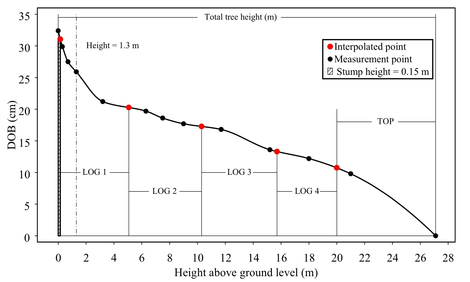
Fig.6 An example of a tree with DBHOB,total tree height and overbark taper measurements(solid dots)being cut into 4 logs in the cut-tolength simulations.The cutting pattern was based on that of its most similar tree selected from among the 13644 stems in the harvester dataset.Log end diameters(red dots)were derived from the taper measurements through PCHIP(see text).In addition to log length and diameters,the length of the top section was generated from the simulations for the estimation of total tree height from harvester data
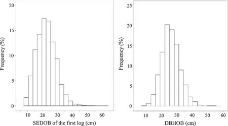
Fig.7 Frequency distributions of SEDOB of the first log and the estimated DBHOB of the 13644 stems in the harvester dataset from which log cutting patterns were extracted for the cut-to-length simulations
In the second step,DBHOB and the estimated total log length of each tree in the taper data set were compared with that of every stem in the harvester data in order to select the most similar stem for the tree.A similarity index(SI)was calculated for each stem as follows:

where DHand LHrepresent the estimated DBHOB and the total log length of a stem in the harvester data set,while DTand LTstand for the DBHOB and the estimated total log length of the tree in the taper data set.The stem with the smallest value of SI among the 13,644 stems was selected as the most similar stem for the taper tree.Even so,the total log length of the most similar tree(LH)still differed from that of the taper tree(LT)as the taper samples were selected from across the state over a much wider diameter and height range than the trees contained in the harvester data (Figs.2 and 7).The difference,calculated as ΔL=LT-LH,varied from-2.2 to 16.0 m,but its distribution was extremely positively skewed,with the first percentile at-1.1 m,the 5th percentile at-0.3 m,a median of zero,and the 90th,95th and 99th percentiles at 1.6,5.3 and 9.8 m,respectively,among the 3099 taper trees used in the CTL simulations.
Because of these differences,some adjustment was made in the third step to the cutting pattern of the most similar tree before it was applied to the corresponding taper tree in the CTL simulations.In doing so,ΔL was evaluated against the range of log length for pulpwood,which varied from 3.6 to 6 m as speci fied by forest management and also shown by the harvester data.For trees with ΔL greater than or equal to 3.6 m,one or more pulp logs were cut above the last cutting height of the most similar stem to a length within the speci fied range in a way to minimize wastage.For trees with ΔL greater than 0 and less than 3.6 m,ΔL was added to the length of the top log of their most similar trees to form a longer section,which was then cut up in the same way as described above.For a small number of taper trees with ΔL<0,but mostly greater than-1 m,the top log of their most similar trees was shortened by ΔL.If the shortened length was equal to or greater than 3.6 m,it was taken as the length of the last log in the CTL simulations.Otherwise,the procedure described above for trees with ΔL greater than 0 and less than 3.6 m was repeated again.Following these adjustments,the difference between the estimated log length LTand the total log length actually realized in the simulations varied from 0 to a maximum of 1.2 m among the 3099 taper trees.The adjusted cutting patterns left little wastage in the top section of the taper trees in the simulations but kept any waste section that was cut from the lower stem of their most similar trees.In doing so,the simulated cutting patterns remained the most realistic,unlike some CTL and bucking-to-value simulations that used modelled taper curves(Malinen et al.2007).In the final data set generated by the CTL simulations,SEDOBTLranged from 3.9 to 20.4 cm with a median of 12.1 cm and the minimum total log length was 4.2 m,while the length of the top section varied from 1.2 to 14.0 m,with a median of 5.9 m,but the length of 90%of the top sections was between 3.0 and 8.8 m.
Using the adjusted cutting pattern for each taper tree,the cutting points were located on its interpolated stem pro file and then the interpolated DOB values were obtained in the fourth step.Finally,in the fifth step,the values of stump height,log number,length,LEDOB and SEDOB,and the length between the last cut to the tip of the tree were exported to a holding data set for further analysis(Fig.5).All steps of the CTL simulations were completed using a computer program written in C#.
Estimating total tree height
The data set generated from the CTL simulations of 3099 taper trees was randomly split into two parts,one containing 2099 trees for developing an equation to estimate total tree height and the other containing 1000 trees for testing its accuracy.Varjo(1995)formulated a model to predict the length of the top section of a tree that was not commercially harvested and processed by the harvester head for pine,spruce and birch species in Finland.The three predictor variables of this model included DBHOB,the total log length and the small end diameter underbark(SEDUB)of the top log.This model form was adopted for P.radiata after replacing the SEDUB with SEDOBTL(i.e.,the SEDOB of the top log)in the model as shown below:

where Ltoprepresents the length of the top section in meters,L is the total log length in meters,DBHOB and SEDOBTLare in centimeters,and ε is the error term assumed to follow a normal distribution with zero mean.The parameters were estimated through ordinary least squares regression.The residuals from regression were examined by using both diagnostic plots and statistical tests to detect possible violations of the normality assumption.The diagnostic plots consisted of four plots:the observed stem volume plotted against fitted values with the line of unity,the corresponding residual plot,the normal quantile–quantile plot and the frequency distribution of the residuals.To correct for log transformation bias,Snowdon’s(1991)bias correction factor was calculated following parameter estimation.Using the estimated Ltop,the predicted total tree height was calculated as follows:

To provide an alternative benchmarking comparison,total tree height was obtained from the overbark taper equation for P.radiata of Zhang et al.(2015)through a numerical search routine.This taper equation adopted the trigonometric variable-form taper model of Bi(2000),and its parameters were estimated using the same data as in Bi and Long(2001).The trigonometric variable-form taper model has been implemented in both commercial software and in-house forest resource management and decision support systems in Australia and New Zealand.As DOB at any height above ground level could be obtained through the equation of Zhang et al.(2015)for a given pair of DBHOB and total tree height,an intuitive but naive approach of estimating the total height of a tree with a given DBHOB and several values of DOB at log ends as in the form of harvester data would be to search for a particular total tree height that could best approximate the DOB values from a complete range of all possible total heights for the DBHOB.
To help de fine this search range,the three-parameter Chapman-Richards function was used:

where H stands for total tree height in m,D is DBHOB in cm,and a,b,and c are parameters that will be estimated using quantile regression.This function had been shown to provide a more satisfactory fit to height and diameter data than many alternative model forms by Huang et al.(1992,1999)and Bi et al.(2000,2012).Two extreme nonlinear conditional quantile curves,the 0.005th and the 0.995th,in the form Eq.(11)were estimated using the R package quantreg,and the total tree height and DBHOB values of the 3165 trees in the taper dataset(Fig.2).For a tree with a given DBHOB,the search range was then de fined by the lower and upper quantile curves.A computer program was written to start the search from the minimum total tree height as determined by the lower quantile curve for the given DBHOB,and then to proceed with an increment of 0.1 m each time afterward until the maximum total tree height as determined by the upper quantile curve was reached.At each step of the search,a corresponding MSEP was calculated using the observed and estimated values of DOB in the way as shown in Eq.(5).The height that gave the smallest MSEP among all the searched heights was selected to be the estimated total tree height for the tree(Fig.8).This numerical search routine was carried out to obtain another set of total height estimates for the 1000 trees in the testing data set.The accuracy of these estimates was compared with that of Varjo’s model in Eq.(10)through the four benchmarking statistics as shown in Eqs.3–6.
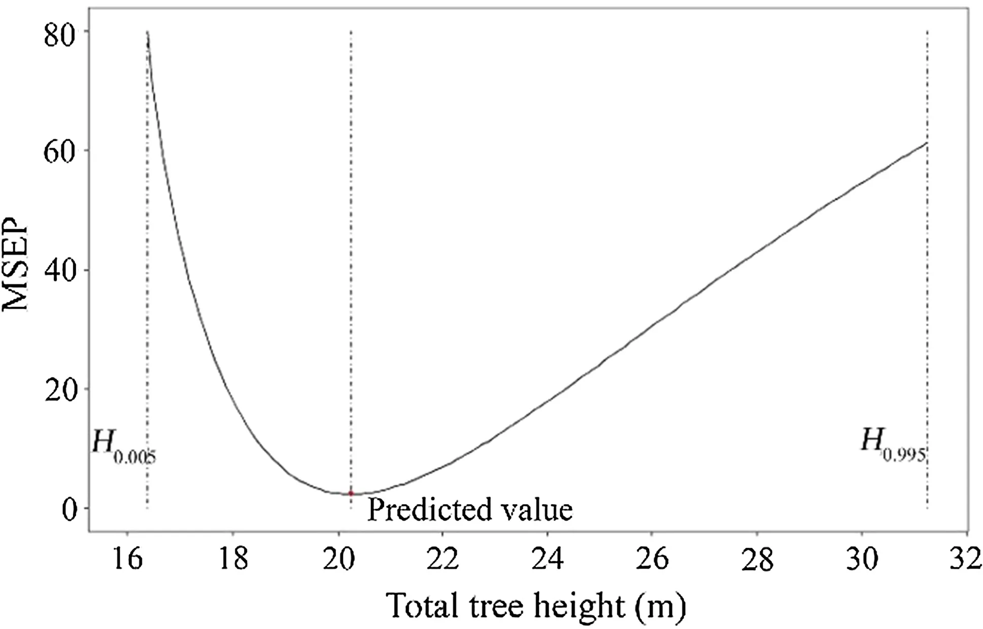
Fig.8 An example of the changes in MSEP as the value of total tree height inputted into the taper equation increased from the smallest value(H0.005)at the start of the numerical search routine,with an increment of 0.1 m at each step,to the largest value(H0.995)at the end of the search.H0.005and H0.995represent the 0.005th and 0.995th conditional quantiles of total tree height for any given DBHOB(see Fig.2).The height with the smallest MSEP was selected to be the predicted total tree height as indicated by the vertical line in the middle
This comparison evaluated the global predictive performance of the two approaches across all 1000 trees but not the local performance within any subspace of the data.For a more local evaluation,the entire data space of 1000 trees was divided into subspaces in three ways.First,the data were divided into four size classes according to DBHOB and tree height in a manner similar to that of Flewelling and Raynes(1993)and Bi(2000).The 0.50th nonlinear height–diameter quantile curve in the form of Eq.(11)was obtained using the R package quantreg;this median curve divided the 1000 trees into two halves,i.e.,relative taller and shorter trees for a given DBHOB.Then the trees in each half were further divided into two parts depending on their diameter being smaller or larger than the median DBHOB.In this way,the 1000 trees were divided into four size classes,each having about a similar number of trees(Fig.9).Second,the total log length of each tree was divided by its total tree height to obtain a log length ratio(Rl),which ranged from 0.46 to 0.88 among the 1000 trees.Because there were a total of 26 trees with Rlbelow 0.6 and only two trees with Rlbelow 0.5,this range was divided into three intervals:(1) Rl≤0.7,(2)0.7<Rl≤0.8 and(3)Rl> 0.8,containing 269,530 and 201 trees,respectively.Third,the data were divided into seven groups according to the total number of logs cut from each stem which ranged from 1 to 9.Finally,the four benchmarking statistics as described above were calculated for both the Varjo’s model and the taper function over all subspaces of data to compare their local predictive performances.
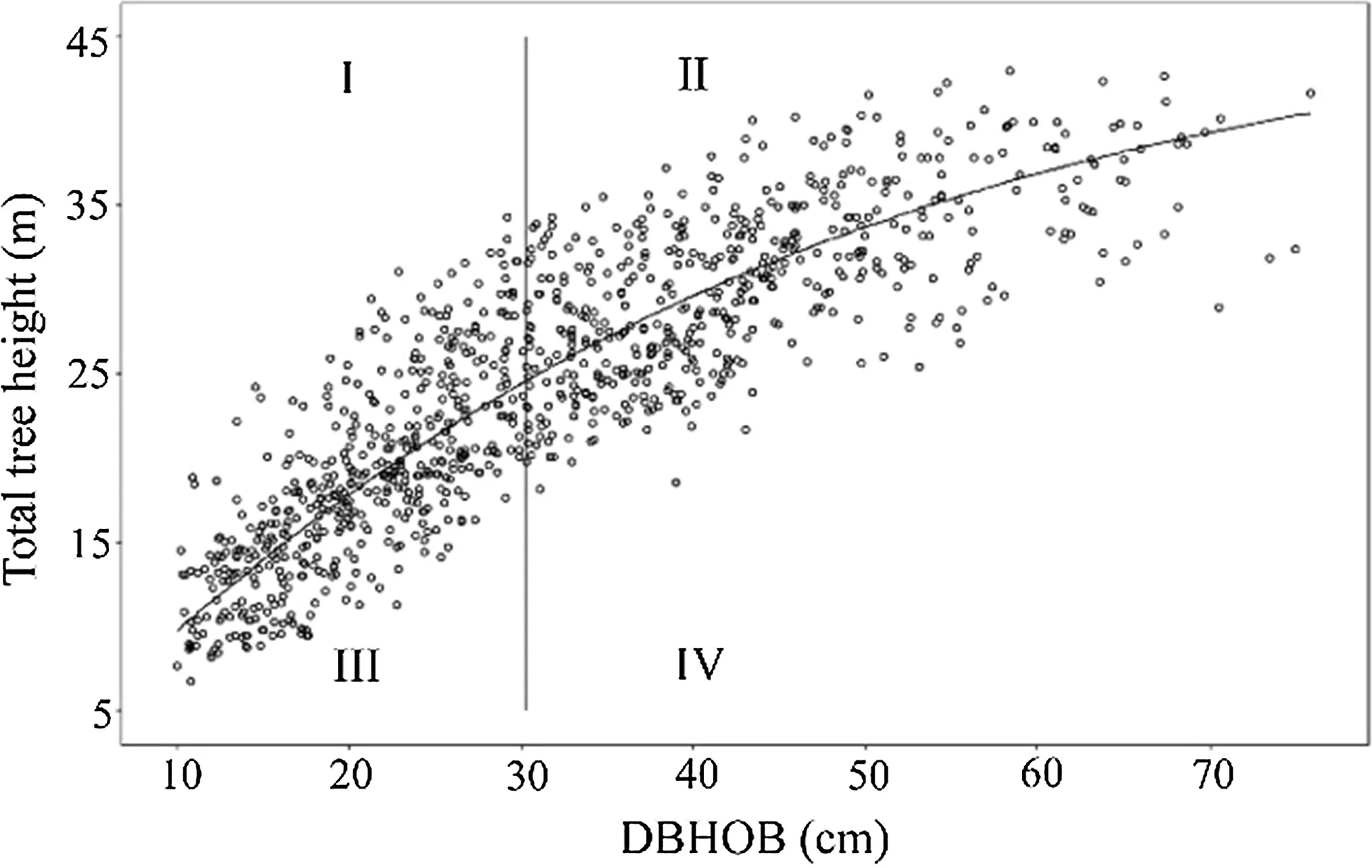
Fig.9 Total tree height plotted against DBHOB for the 1000 trees in the testing dataset.The entire data space was divided into four subspaces by the 0.50th nonlinear conditional height-diameter quantile curve and the median of DBHOB
Results
As shown in Fig.3,the average stump height over all 31 sites was 15 cm,but there was a large degree of variation across the 31 sites.At any particular site,stump height could vary from less than 10 cm to more than 50 cm in the extreme cases.Among the 31 sites,the average stump height varied from 8.2 to 24.4 cm with a median of 15.6 cm,while the median stump height varied from 7 to 24 cm with a median of 13 cm.In comparison,the 90th percentile of stump height varied from 15 to 32 cm across these sites.
Converting DOB at any height below 3 m to DBHOB
There were little differences between the OLS and SUR estimation in the calculated values of MSEP for DBHOB conversion using Eqs.2 and 5 for most of the 30 speci fied heights.However,the OLS estimation had slightly smaller values of MSEP for heights between 2 and 3 m,therefore the OLS parameter estimates of the system of 30 equations were reported here.The estimated parameters and the calculated Snowdon’s bias correction factors for the system of 30 equations as speci fied in model(1)changed systematically as height increased from 0.05 to 2.95 m with an even interval of 0.1 m(Table 1).The estimated value of α gradually increased from nearly-0.32 at 0.05 m to about zero at 1.35 m,just above the de fined breast height of 1.3 m,and finally to 0.26 at the height 2.95 m.As α increased,the estimated value of β decreased from 1.04 at 0.05 m to almost 1 at 1.35 m,and finally to 0.96 at 2.95 m.The calculated bias correction factor was almost 1 in the close neighborhood of breast height.As height moved further away from breast height,it became increasingly larger and reached 1.001 at the two ends of the height range of 0.05 and 2.95 m.The mean squared error for the equations was the largest at the base height of 0.05 m,the smallest in the close neighborhood of breast height,and became increasingly larger again as height increased further above breast height.
These parameter estimates and bias correction factors in Table 1 were for the 30 speci fied heights only.Through simple linear or the nearest interpolation,parameters and correction factors were obtained for the estimation of DBHOB atany otherheightwithin therangeof 0.05–2.95 m.The simple linear interpolation had little bias across the height range as shown by the values of MEP,while the nearest interpolation had slightly larger but still negligible bias in the estimation of DBHOB(Fig.10).For both interpolation methods,the benchmarking statistic MAEP,i.e.,the average size of error in the estimation of DBHOB,was within 1 cm except for the first three heights below 0.3 m.It followed a V-shaped pattern across the height range,with the smallest value sitting in between 1.25 and 1.35 m.Correspondingly,MSEP followed similar patterns across the height range for both interpolation methods.
Converting SEDOB of the first log to DBHOB
Parameter estimates and fitting statistics for the 46 equations that were used to convert SEDOB of the first log to DBHOB again showed systematic changes as height increased from 3.05 to 9.55 m(Table 2),continuing the trends shown in Table 1 for height from 0.05 to 2.95 m.The parameters of the 0.50th nonlinear conditional quantile curve in the form of Eq.(7)estimated by the R packagequantreg were 3.05 and-16.89 for a and b respectively.This curve was used for estimating the small end diameter overbark of the top log,SEDOBTL,of a taper tree from its DBHOB before calculating its total log length in the first step ofCTL simulations.According to thiscurve,SEDOBTLincreased from 4 to 17 cm as DBHOB increased from 10 to 80 cm,i.e.,the complete diameter range of taper trees.The three parameters of the Chapman–Richards function(Eq.11)were a=31.6,b=0.0315,c=1.6997,for the 0.005th quantile(H0.005)and a=49.6,b=0.0281,c=0.7078 for the 0.995th quantile(H0.995).The two extreme conditional quantile curves de fined the range of total tree height for any given DBHOB in the numerical search routine for the most likely estimate through the trigonometric variable-form taper equation(see Fig.2).For example,the search range determined by the pair of extreme quantiles(H0.005,H0.995)in meters were(10.0,28.6),(22.6,41.9)and(28.7,47.1)for DBHOB equal to 20,50 and 80 cm,respectively.
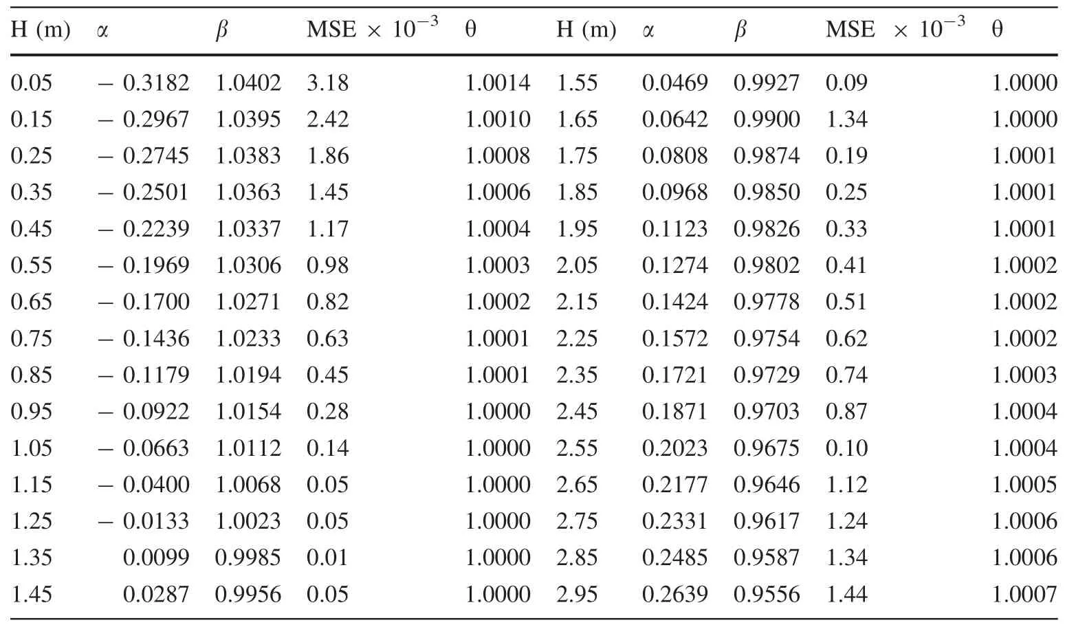
Table 1 Parameter estimates and Snowdon’s bias correction factors(θ)for the 30 heights(H)below 3 m above ground level as speci fied in model(1).Data from all 3165 trees contained in the taper dataset were used in the estimation.The values of R2for the equations were 0.98 for the lowest two heights of 0.05 and 0.15 m,and 0.99 or greater for all other heights

Fig.10 Comparative accuracy in estimating the DBHOB of 3165 trees using the conversion coef ficients and bias correction factors derived through simple linear and the nearest interpolations at the 29 heights that were randomly selected from within the 29 even intervals between 0.05 and 2.95 m(see text)
Estimating total tree height
The six estimated parameters of Varjo’s model in Eq.(9)were all signi ficantly different from zero,and the model explained about 61%of the variation in the log transformed Ltopas indicated by a t test for parameter estimates and the value of R2for the ordinary least squares regression(Table 3).The calculated bias correction factor was 1.0208.The more or less even spread of the residuals when plotted against the predicted values did not suggest the presence of heteroskedasticity(Fig.11).However,the residual normal quantile plot showed that the residualdistribution had a slight departure from normality,which was con firmed by the Kolmogorov–Smirnov test at α =0.05 level.The distribution was not mesokurtic,but symmetric leptokurtic as the skewness of the residual distribution was only-0.06,almost zero and the kurtosis was 4.42,larger than 3,the kurtosis of any univariate normal distribution.The 5th and the 95th percentile of the residual distribution were-0.33 and 0.34,equal to 0.7 and 1.4 m after back-transformed from logarithm(Fig.11).The predicted ln Ltopwas back-transformed from logarithm,corrected for log-transformation bias,and included in Eq.(10)for the prediction of total tree height.
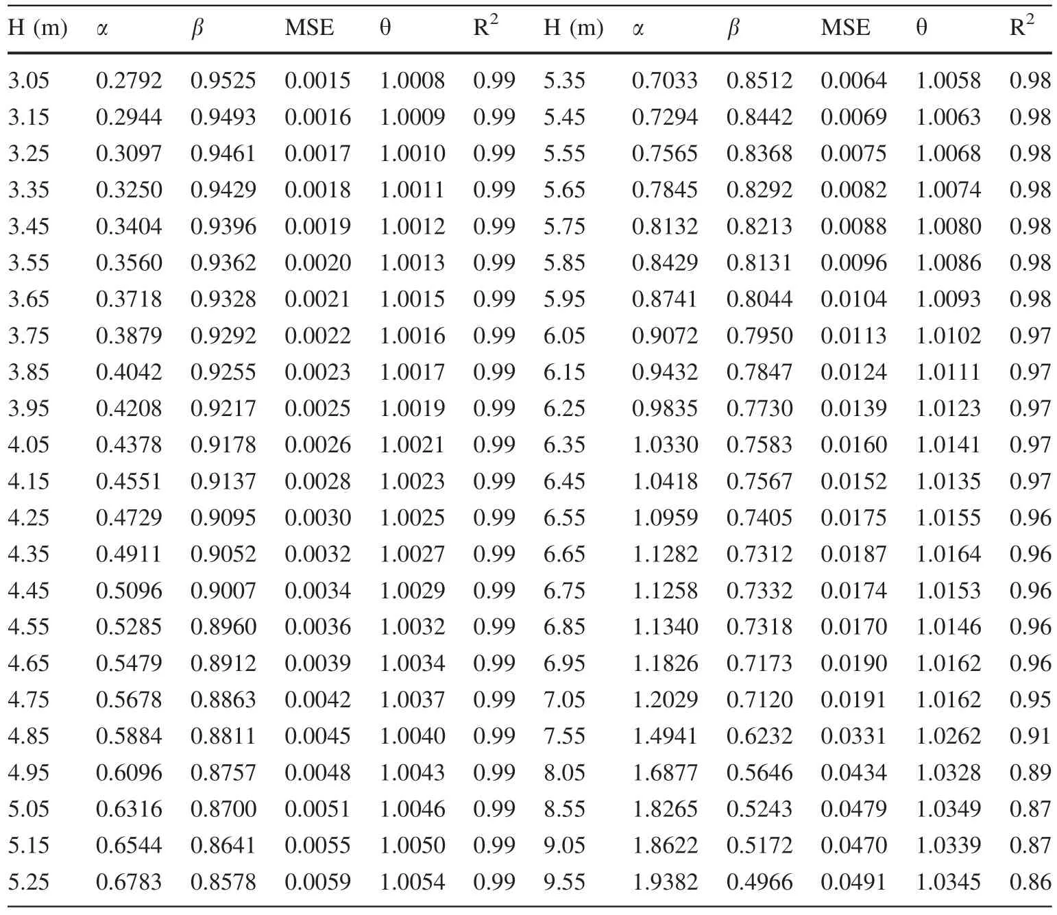
Table 2 Parameter estimates,fitting statistics and Snowdon’s bias correction factors(θ)for the system of 46 equations used to convert DOB to DBHOB at each speci fied height(H)above ground level
The benchmarking statistics calculated for Eq.(10)using the 1000 trees in the testing data set showed that there was little bias in its prediction of total tree height because the calculated value of MEP was-0.01 m.The average size of the prediction error was 0.93 m as indicated by the value of MAEP,and 90%of the prediction errors fell between-1.8 and 2.1 m.The value of MSEP was 1.60,and the prediction coef ficient of determination(R2p)was 0.98(Fig.12).In comparison to Eq.(10),there was a small bias of-0.10 m in the total tree height prediction obtained through the numerical search routine using the trigonometric variable-form taper function.The value of MAEP was larger,about 1.2 m,and 90%of the prediction errors fell between-2.5 and 2.5 m.MSEP was 2.41,also larger,and R2pwas 0.96,slightly smaller(Fig.12).This comparison showed the comparative predictive performance of the two approaches globally across all 1000 trees.
When the entire data space of 1000 trees was divided into subspaces for a more local evaluation,greater differences in predictive performance emerged between the twoapproaches.First,over the four subspaces of data separated by the median height–diameter curve and the median DBHOB in Fig.9,Varjo’s model showed a systematic pattern of bias in total tree height prediction.It underestimated the total tree height of relatively slenderer trees that were above the median height–diameter curve in subspace I and II but overestimated that of the relatively squatter trees below the curve(Fig.13).Either way,the bias was small,within±0.31 m.In comparison,the numerical search routine tended to overestimate the total height of trees in subspace I and IV(i.e.,smaller slender trees and larger squatter trees)by about 0.2 m,and it was almost unbiased for trees within subspace II and III as the values of MEP were about± 0.1 m.Except for MEP,Varjo’s model was superior to the numerical search routine as it had smaller MAEP and MSEP but largerthan the taper function(Fig.13).Secondly,across the three log length ratio (Rl)intervals,the bias was the smallest when 0.7<Rl≤0.8,with MEP approaching -0.12 and-0.32 m for Varjo’s model and the numerical search routine,respectively(Table 4).The values of MAEP and MSEP were also the smallest,and the correspondingwas the largest for both approaches,being 0.98 and 0.97 for Varjo’s model and the numerical search routine.For the other two log length ratio intervals with Rl≤0.7 and Rl>0.8,MEP was much larger in size,being 0.91 and-0.94 m for Varjo’s model and 1.18 to-1.24 m for the numerical search routine.The values of MAEP and MSEP were also larger and,correspondingly,the values ofwere smaller,being 0.93 and 0.95 for Varjo’s model and 0.91 and 0.93 for the numerical search routine.Again,Varjo’s model was superior to the numerical search routine across all three intervals(Table 4).Third,among the seven groups of the number of logs cut from each stem,MEP varied between-0.14 to 0.12 m for Varjo’s model,and between-0.67 to 0.29 m for the numerical search routine.The values MAEP and MSEP were much larger,and those forwere much smaller for the numerical search routine(Table 5).

Table 3 Parameter estimates,their standard errors in brackets and Snowdon’s bias correction factor(θ)for Varjo’s model in Eq.(9)
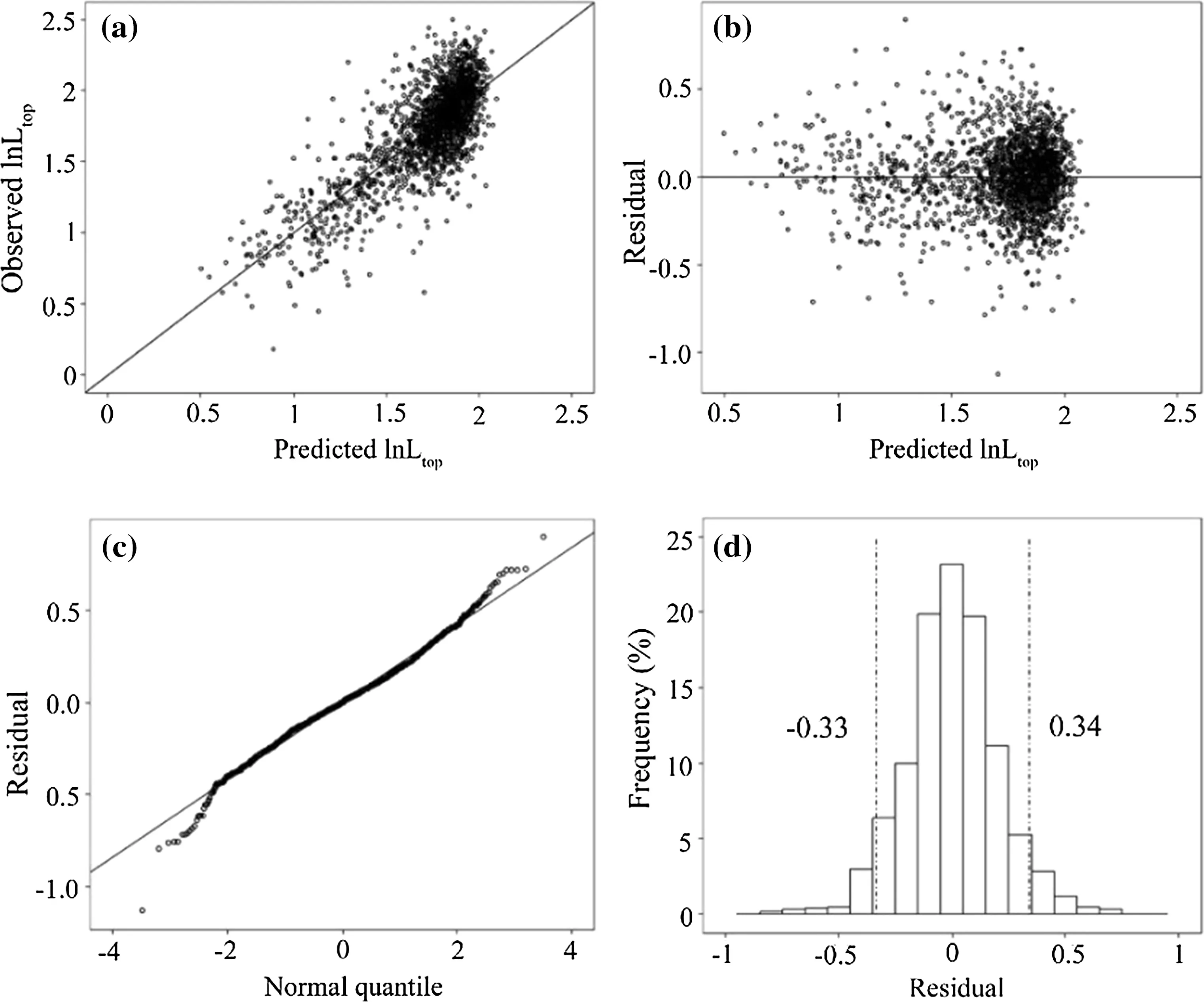
Fig.11 Diagnostic plots of ordinary least squares regression for Varjo’s model in Eq.(9):a observed lnLtop plotted against predicted values with a line of unity;b residual plot;c residual quantile–quantile plot;d residual frequency distribution with two vertical lines indicating the 5th and the 95th percentiles of the distribution
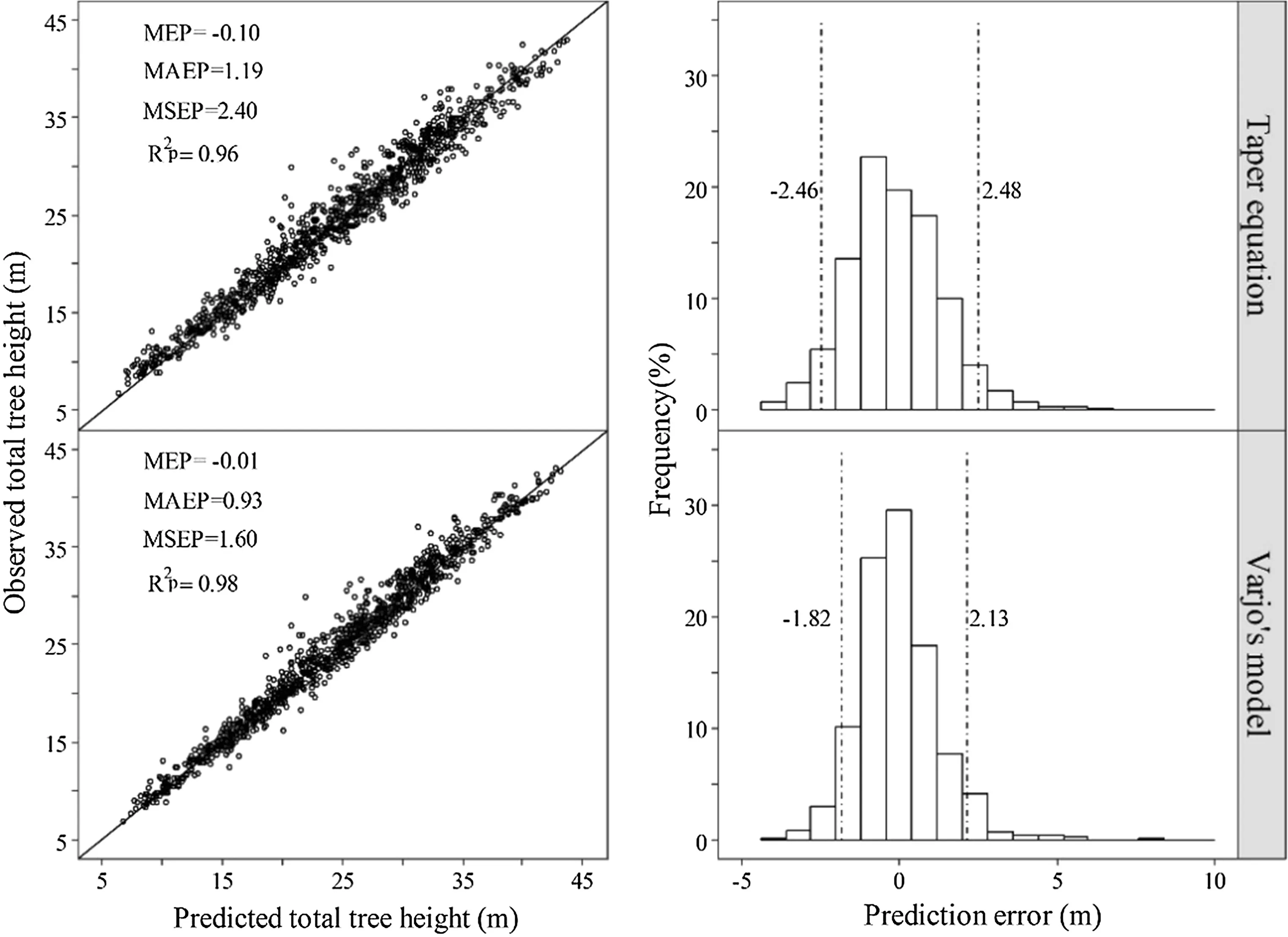
Fig.12 Observed total tree height plotted against predicted values with a line of unity for Varjo’s model and the variableform trigonometric taper equation(left)and the corresponding frequency distributions of prediction error with two vertical lines indicating the 5th and the 95th percentiles of the distribution(right)
Discussion
The extent of variation in stump height within and across sites(Fig.3)could be attributed to several factors.The design of the harvester head in the distance from the base of the head to the saw determines the minimum achievable stump height.Debris such as rocks and logs at the base of a tree may prevent a machine operator from felling the tree at a height close to the ground level because harvester heads are not designed to clear the debris.Felling trees on a slope tend to leave stumps that are higher on the downhill side.There were also differences in the skill and behavior of operators,and some might be better than others at keeping stumps short during harvesting.Double leaders and stem deformity or defects such as severe butt swell or sweep just above the base of a tree might force operators to cut a stump higher rather than to fell the tree closer to the ground level and to cut to waste a swept butt.Doing so would also avoid the need for a second cut.
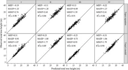
Fig.13 Observed total tree height plotted against estimated values with a line of unity for Varjo’s model and the variable-form trigonometric taper equation over the four subspaces of data(see Fig.9)

Table 4 Benchmarking statistics of prediction accuracy of total tree height for Varjo’s model and the variable-form trigonometric taper equation across the three total log length ratio classes

Table 5 Benchmarking statistics of prediction accuracy of total tree height for Varjo’s model and the variable-form trigonometric taper equation over 7 groups of trees where the number of logs including waste sections cut from each stem ranged from 1 to 9
As reviewed by Pond and Froese(2014),many equations have been developed to predict DBHOB from stump dimensions for a large number of coniferous and broadleaved species in different forest types over the past 60 years for the reconstruction of preharvest stems and stand structures from postharvest data.These equations were based either on a constant stump height,as in the case of Corral-Rivas et al.(2007)or on a narrow range of variation in stump height(e.g.,Bylin 1982;Westfall 2010;Pond and Froese 2014).The system of 30 equations developed in this study enables the estimation of DBHOB from DOB measured at any height below 3 m above ground level for P.radiata through simple linear or the nearest interpolation of the estimated parameters and bias correction factors.These equations will be applicable in cases where DBHOB was not directly measured,recorded or extrapolated by the harvester head during tree felling and log cutting.Even when DBHOB was measured and recorded,the accuracy of the machine measurements may need to be validated,and the recorded values may need to be adjusted or corrected if necessary.For example,unpublished data obtained by the second author from 100 southern pine trees with DBHOB ranging from 22 to 48 cm that were carefully cut for a wood quality study in northern NSW showed that the harvester head substantially underestimated DBHOB.The underestimation ranged from 1.7 to 8.8 cm,with a mean and a median of 4.1 and 4.2 cm.The range represented 5–25%of the observed DBHOB.There are a number of possible causes of harvester head diameter measurement errors,including use of the incorrect bark function,penetration or stripping of the bark during processing and poor harvester head calibration(Strandgard and Walsh 2012).In such cases,the system of equations can be applied to adjust or to correct the machine measured DBHOB by using stump dimensions from postharvesting surveys,the height above stump of the first DOB measured by the harvester head or the height of DBHOB measurement speci fied in the production instruction file of the harvester.Besides its application in the processing of harvester data,the system of equations can be used to reconstruct the sizes of individual trees and structures of stands directly from stump height and diameters.It can also be used to convert diameter measurements taken at different breast heights,e.g.,from 1.4 to 1.3 m.In doing so,it was proved to be slightly more accurate than the conversion factor of Zhang et al.(2015).
Although the system of equations and the interpolation algorithms can be easily programmed and implemented,a potential drawback of the system of equations may still be the perceived inconvenience associated with the number of equations.Because the two estimated parameters and the bias correction factor changed systematically but nonlinearly with height above ground level as shown in Table 1,attempts were made to smooth the discrete values of each parameter into a continuous polynomial function of height within the de fined range of 0.05 to 2.95 m.However,for all degrees of polynomials from low to high that were explored,local bias in parameter prediction over a certain height range persisted for all three parameters.As a result,the attempted estimation of DBHOB through parameter prediction from the continuous polynomial functions was not as accurate as the estimation though simple linear interpolation and the nearest interpolation as previously described.Eventually,this parameter prediction approach was abandoned.As also recognized by Pond and Froese(2014),an alternative single equation approach based on the neiloidal segment of a taper function for the lower stem may need to be explored in future research.
Varjo’s(1995)equations for predicting the length of the top part of the stem(Ltop)were originally developed for pine,spruce and birch trees in Finland and were applicable to stems with the small end diameter of the top log(SEDUBTL)between 5 and 10 cm and the minimum log length of 1.5 m.His predictive equations have proved useful in reconstructing individual trees from harvester data(e.g.,Palander et al.2009;Vesa and Palander 2010;Siipilehto et al.2016).Equation(9)for predicting Ltopof P.radiata was based on Varjo’s(1995)model but with SEDUBTLreplaced by SEDOBTLas a predictor.The value of SEDOBTLranged from 3.9–19.6 cm,and the minimum log length was 4.2 m among the 2099 trees used in estimating the parameters of Eq.(9).This range of SEDOBTLwas much wider and the minimum log length much greater than that stated for Varjo’s(1995)equations.The estimated Eq.(9)explained 61%or the variation in Ltopas indicated by the value of R2in Table 3,but this fit statistic was not reported by Varjo(1995)for his equations.
However,when the predicted Ltopwas added to total log length and stump height in Eq.(10),the predicted total tree height was unbiased and the prediction coef ficient of determination(R2p)was 0.98,much greater than 0.61(Fig.11).As shown by the benchmarking results using the 1000 trees in the testing data set,the average size of prediction error and MSEP were 0.93 m and 1.60,respectively,and 90%of the prediction errors were between-1.8 and 2.1 m.This predictive performance was superior to that of the numerical search routine through the trigonometric variable form taper equation,although the latter used all log length and end diameter data generated from the simulated cutting of each stem in the search.The benchmarking statistics of both approaches were compared with the diagnostic plots, fit and validation statistics of conventional height–diameter equations for P.radiata reported in the literature(e.g.,Sánchez et al.2003;Dorado etal.2006).Thecomparisonssuggested thatboth approaches when used with harvester data would outperform the conventionalequations even when they incorporated stand age and the average height and diameter of dominant trees in the stand as predictors.
Varjo’s model underestimated the total tree height of relatively slenderer trees but overestimated that of relatively squatter trees(Fig.13).This systematic pattern of bias in total tree height prediction suggested that prediction accuracy might be improved by incorporating some measure of slenderness into the equation in future research.Over the three log length ratio intervals,Varjo’s model was the least biased and the most precise for the interval in the middle where 0.7<Rl≤0.8.This range included 53%of the 1000 trees in the testing data set and would also be the case for the majority of trees during the final harvesting of plantations based on operational experience.If there were no predictive models available for estimating total tree height from harvester data,the numerical search routine would be an obvious method to use as its prediction accuracy would still be superior to that of the conventional height–diameter equations.
Tree and stand reconstructions of the harvested forest have been well recognised and demonstrated as the necessary first step to provide the essential link of harvester data to conventional inventory,remote sensing imagery and LiDAR data(e.g.,Kiljunen 2002;Maltamo et al.2010;S?derberg 2015;Siipilehto et al.2016).The biometric functions developed in this study have enabled the reconstruction of not only individual trees but also stands and forests of postharvest P.radiata plantations from harvester data.They will provide such a linkage for the most effective combined use of harvester data in predicting the attributes of individual trees,stands and forests,and product recovery for the management and planning of P.radiata plantations in New South Wales,Australia.However,as illustrated by Holopainen et al.(2010)and Westfall and McRoberts(2017)in their studies,when applying these equations,the variation in stump height between and within harvested sites(Fig.3)will need to be kept in mind as it represents a source of uncertainty in the estimation of both DBHOB and total heights.The site-speci fic variation in stump height may need to be examined and quanti fied to reduce the uncertainty and maintain the accuracy of estimation.At the same time,operators of CTL harvesters can be encouraged or required by forest management to leave stumps with a more uniform and lower stump height within and across the harvesting sites.
AcknowledgementsWe thank Mr.Mike Sutton of the Forestry Corporation of NSW for providing the data license to Beijing Forestry University for this collaborative work.We are indebted to the past and present forestry staff of the Forestry Commission of NSW,State Forests of NSW,Forests NSW,and the Forestry Corporation of NSW who collected the data in the field.Michael Mclean and Jan Rombouts provided valuable comments which improved the quality of the manuscript.
Open AccessThis article is distributed under the terms of the Creative Commons Attribution 4.0 International License(http://crea tivecommons.org/licenses/by/4.0/),which permits unrestricted use,distribution,and reproduction in any medium,provided you give appropriate credit to the original author(s)and the source,provide a link to the Creative Commons license,and indicate if changes were made.
Arlinger J,Nordstr?m M,M?ller JJ(2012)StanForD 2010:modern communication with forest machines.Arbetsrapport 784,Skogforsk,Uppsala
Barth A,Holmgren J(2013)Stem taper estimates based on airborne laser scanning and cut-to-length harvester measurements for preharvest planning.Int J For Eng 24(3):161–169
Barth A,M?ller JJ,Wilhelmsson L,Arlinger J,Hedberg R,S?derman U(2015)A Swedish case study on the prediction of detailed product recovery from individual stem pro files based on airborne laser scanning.Ann Sci 72(1):47–56
Baskerville GL(1972)Use of logarithmic regression in the estimation of plant biomass.Can J For Res 2(1):49–53
Bi H(2000)Trigonometric variable-form taper equation for Australian eucalypts.For Sci 46(3):397–409
Bi H,Long YS(2001)Flexible taper equation for site-speci fic management of Pinus radiata in New South Wales Australia.For Ecol Manag 148(1):79–91
Bi H,Jurskis V,O’Gara J(2000)Improving height prediction of regrowth eucalypts by incorporating the mean size of site trees in a modi fied Chapman-Richards equation. Australian For 63(4):257–266
Bi H,Fox JC,Li Y,Lei YC,Pang Y(2012)Evaluation of nonlinear equations for predicting diameter from tree height.Can J For Res 42(4):789–806
Bylin CV(1982)Estimating dbh from stump diameter for 15 southern species.New Orleans,LA:US Department of Agriculture,Forest Service,Southern Forest Experiment Station.Research Note SO-286,p 3
Corral-Rivas JJ,Barrio-Anta M,Aguirre-Calderón OA,Diéguez-Aranda U(2007)Use of stump diameter to estimate diameter at breast height and tree volume for major pine species in El Salto,Durango(Mexico).Forestry 80(1):29–40
Dorado FC,Diéguez-Aranda U,Anta MB,Rodríguez MS,Gadow KV(2006)A generalized height–diameter model including random components for radiata pine plantations in northwestern Spain.For Ecol Manag 229(1):202–213
Downham R,Gavran M(2017)Australian plantation statistics 2017 update.Australian Government Department of Agriculture and Water Resources. Available at agriculture.gov.au/abares/publications
Flewelling JW,Pienaar LV(1981)Multiplicative regression with lognormal errors.For Sci 27(2):281
Flewelling JW,Raynes LM(1993)Variable-shape stem-pro file predictions for western hemlock.Part I.Predictions from DBH and total height.Can J For Res 23(3):520–536
Gerasimov Y,Seliverstov A,Syunev V(2012)Industrial round-wood damage and operational ef ficiency losses associated with the maintenance of a single-grip harvester head model:a case study in Russia.Forests 3(4):864–880
Gerasimov Y,Sokolov A,Syunev V(2013)Development trends and future prospects of cut-to-length machinery.Adv Mater Res 705:468–473
Heinimann HR(2001)Productivity of a cut-to-length harvester family—an analysis based on operation data.In:J.Wang,M.Wolford and J.McNeel(eds),Appalachian hardwoods:managing change,Proceeding of 24th Annual Meeting of the Council on Forest Engineering,July 15–19,Snowshoe,West Virginia,USA,pp 121–126
Heinimann HR(2007)Forest operations engineering and management–the ways behind and ahead of a scienti fic discipline.Croat J For Eng 28(1):107–121
Hellstr?m T,L?rkeryd P,Nordfjell T,Ringdahl O(2009)Autonomous forest vehicles:historic,envisioned,and state-of-the-art.Int J For Eng 20(1):31–38
Holmgren J,Barth A,Larsson H,Olsson H(2012)Prediction of stem attributes by combining airborne laser scanning and measurements from harvesters.Silva Fennica 46(2):227–239
Holopainen M,Vastaranta M,Rasinm?ki J,Kalliovirta J,M?kinen A,Haapanen R,Melkas T,Yu X,Hyypp?J(2010)Uncertainty in timber assortment estimates predicted from forest inventory data.Eur J For Res 129(6):1131–1142
Huang SM(1999)Ecoregion-based individual tree height-diameter models for lodgepole pine in Alberta.West J Appl For 14(4):186–193
Huang SM,Titus SJ,Wiens DP(1992)Comparison of non-linear height-diameter functions for major Alberta tree species.Can J Res 22(9):1297–1304
Huang SM,Yang Y,Wang Y(2003)A critical look at procedures for validating growth and yield models.In:Amaro A,Reed D,Soares P(eds)Modelling Forest Systems.CABI Publishing,Oxford,pp 271–293
Huyler NK,LeDoux CB(1999)Performance of a cut-to-length harvester in a single-tree and group selection cut.USDA Forestry Service,Northeastern Research Station,Research Paper NE–711,p 6
Kiljunen N(2002)Estimating dry mass of logging residues from final cuttings using a harvester data management system.Int J For Eng 13(1):17–25
Koenker R(2015)Quantreg:Quantile Regression.R package version 5.19. Available at: https://CRAN.R-project.org/package=quantreg
Koenker R.(2016).quantreg:quantile regression.R package version 5.27.Available at:https://CRAN.R-project.org/package=quantreg
Koenker R(2017)Quantile regression:40 years on.Annu Rev Econ 9(1):155–176.https://doi.org/10.1146/annurev-economics-063016-103651
Kong JL,Ding XK,Liu JH,Yan L,Wang JL(2015)New hybrid algorithms for estimating tree stem diameters at breast height using a two dimensional terrestrial laser scanner.Sensors 15(7):15661–15683
Koskela L,Nummi T,Wenzel S,Kivinen VP(2006)On the analysis of cubic smoothing spline-based stem curve prediction for forest harvesters.Can J For Res 36(11):2909–2919
Lewis NB,Ferguson IS,Sutton WRJ,Donald DGM,Lisboa HB(1993)Management of radiata pine.Inkata Press Pty Ltd/Butterworth-Heinemann
Malinen J,Kilpel?inen H,Piira T,Redsven V,Wall T,Nuutinen T(2007)Comparing model-based approaches with bucking simulation-based approach in the prediction of timber assortment recovery.Forestry 80(3):309–321
Malinen J,Laitila J,V??t?inen K,Viitam?ki K(2016)Variation in age,annual usage and resale price of cut-to-length machinery in different regions of Europe.Int J For Eng 27(2):95–102
Maltamo M,Bollandsa?s OM,Vauhkonen J,Breidenbach J,Gobakken T,N?sset E(2010)Comparing different methods for prediction of mean crown height in Norway spruce stands using airborne laser scanner data.Forestry 83(3):257–268
Mead DJ(2013)Sustainable management of Pinus radiata plantations.Food and Agriculture Organization of the United Nations,Italy,Room
Miettinen M,Kulovesi J,Kalmari J,Visala A(2010)New measurement concept for forest harvester head.In:Howard A,Iagnemma K,Kelly A(eds)Field and service robotics.Springer,Berlin,pp 35–44
M?ller JJ,Wilhelmsson L,Arlinger J,Moberg L,Sondell J(2003)Automatic characterization of wood properties by harvesters to improve customer orientated bucking and processing.Skogforsk.Arbetsrapport.Nr 537:64–76
Murphy G (2003)Procedures for scanning radiata pine stem dimensions and quality on mechanised processors.Int J For Eng 14(2):11–21
Murphy G,Wilson I,Barr B(2006)Developing methods for preharvest inventories which use a harvester as the sampling tool.Australian For 69(1):9–15
Murphy GE,Acuna MA,Dumbrell I(2010)Tree value and log product yield determination in radiata pine(Pinus radiata)plantations in Australia:comparisons of terrestrial laser scanning with a forest inventory system and manual measurements.Can J For Res 40(11):2223–2233
Nash JE,Sutcliffe JV (1970)River flow forecasting through conceptual models part I—A discussion of principles.J Hydrol 10(3):282–290
Nieuwenhuis M,Dooley T(2006)The effect of calibration on the accuracy of harvester measurements.Int J For Eng 17(2):25–33
Nordfjell T,Bj?rheden R,Thor M,W?sterlund I(2010)Changes in technical performance,mechanical availability and prices of machines used in forest operations in Sweden from 1985 to 2010.Scand J For Res 25(4):382–389
Nummi T,M?tt?nen J(2004)Estimation and prediction for low degree polynomial models under measurement errors with an application to forest harvesters.J Roy Stat Soc 53(3):495–505
?hman M,Miettinen M,Kannas K,Jutila J,Visala A,Forsman P(2008)Tree measurement and simultaneous localization and mapping system for forest harvesters.Field and service robotics.Springer,Berlin,pp 369–378
Olivera A,Visser R,Acuna M,Morgenroth J(2016)Automatic GNSS-enabled harvester data collection as a tool to evaluate factors affecting harvester productivity in a Eucalyptus spp.harvesting operation in Uruguay.Int J For Eng 27(1):15–28
Palander T,Vesa L,Tokola T,Pihlaja P,Ovaskainen H(2009)Modelling the stump biomass of stands for energy production usingaharvesterdatamanagementsystem.BiosysEng 102(1):69–74
Peuhkurinen J,Maltamo M,Malinen J(2008)Estimating speciesspeci fic diameter distributions and saw log recoveries of boreal forests from airborne laser scanning data and aerial photographs:a distribution-based approach.Silva Fennica 42(4):625–641
Pond NC,Froese RE(2014)Evaluating published approaches for modelling diameter at breast height from stump dimensions.Forestry 87(5):683–696
Priddle J(2005)Computer-controlled optimisation in cut-to-length harvesting systems and associated data flows.Available at:https://gottsteintrust.org/reports/
Rasinm?ki J,Melkas T(2005)A method for estimating tree composition and volume using harvester data.Scand J For Res 20(1):85–95
Sánchez CAL,Varela JG,Dorado FC,Alboreca AR,Soalleiro RR,González JGá,Rodríguez FS(2003)A height-diameter model for Pinus radiata D.Don in Galicia(Northwest Spain).Ann For Sci 60(3):237–245
Sellén D(2016)Big data analytics for the forest industry:a proof-ofconcept built on cloud technologies.M.Sc.Thesis,Mid Sweden University
Siipilehto J,Lindeman H,Vastaranta M,Yu X,Uusitalo J(2016)Reliability of the predicted stand structure for clear-cut stands using optional methods:airborne laser scanning-based methods,smartphone-based forest inventory application Trestima and preharvest measurement tool EMO.Silva Fennica,50(3),article ID 1568,Available at:https://dx.doi.org/10.14214/sf.1568
Snowdon P(1991)A ratio estimator for bias correction in logarithmic regressions.Can J For Res 21(5):720–724
S?derberg J(2015)A method for using harvester data in airborne laser prediction of forest variables in mature coniferous stands.M.SC Thesis:Swedish University of Agricultural Science,Uppsala,Sweden,p 31
Spinelli R,Magagnotti N,Picchi G(2011)Annual use,economic life and residual value of cut-to-length harvesting machines.J For Econ 17(4):378–387
Srivastava VK,Giles DE(1987)Seemingly unrelated regression equations models:estimation and inference.CRC Press,Boca Raton,pp 1256–1264
Stendahl J,Dahlin B(2002)Possibilities for harvester-based forest inventory in thinnings.Scand J For Res 17(6):548–555
Strandgard M,Walsh D(2012)Assessing measurement accuracy of harvester heads in Australian pine plantation operations.Cooperative Research Centre for Forestry Technical Report 225,p 15
Strandgard M,Walsh D,Acuna M(2013)Estimating harvester productivity in Pinus radiata plantations using StanForD stem files.Scand J For Res 28(1):73–80
Uusitalo J(2010)Introduction to forest operations and technology.JVP Forest Systems Oy,H?meenlinna
Vanclay JK(2011)Future harvest:what might forest harvesting entail 25 years hence?Scand J For Res 26(2):183–186
Varjo J(1995)Latvan hukkaosan pituusmallit m?nnylle,kuuselle ja koivulle metsurimittausta varten.In:Puutavaran mittauksen kehitt?mistutkimuksia 1989–93(Verkasalo E ed),Finnish Forest Research Institute,Research Papers 558,pp.21–23(in Finnish)
Vesa L,Palander T(2010)Modeling stump biomass of stands using harvester measurements for adaptive energy wood procurement systems.Energy 35(9):3717–3721
Wackerly DD,Mendenhall W,Scheaffer RL(1996)Mathematical statistics with applications.Duxbury Press,Belmont,p 798
Westfall JA(2010)New models for predicting diameter at breast height from stump dimensions.North J Appl For 27(1):21–27
Westfall JA,McRoberts RE(2017)An assessment of uncertainty in volume estimates for stands reconstructed from tree stump information.For:Int J For Res 90(3):404–412
Williams C,Ackerman P(2016)Cost-productivity analysis of South African pine sawtimber mechanised cut-to-length harvesting.South For:J For Sci 78(4):267–274
Zellner A(1962)An ef ficient method of estimating seemingly unrelated regressions and tests for aggregation bias.J Am Stat Assoc 57(298):348–368
Zhang YH,Li Y,Bi H(2015)Converting diameter measurements of Pinus radiata taken at different breast heights.Australian For 78(1):1–5
 Journal of Forestry Research2018年1期
- Journal of Forestry Research的其它文章
- Vascular bundle connection between seed stalk and seed coat of Caragana arborescens
- Robust optimization for volume variation in timber processing
- Modelling the spatial distribution of snake species in northwestern Tunisia using maximum entropy(Maxent)and Geographic Information System(GIS)
- Population and genetic diversity of Tibetan red deer based on fecal DNA
- The distribution and frequency of damage to roadside trees in low-volume road construction
- An evaluation of harvesting costs in present and planned operations:case study—Waston District of Mazandaran Wood and Paper Industries
