Probabilistic Robust Linear Parameter-varying Control of a Small Helicopter Using Iterative Scenario Approach
Zhou Fang,Hua Tian,and Ping Li
Probabilistic Robust Linear Parameter-varying Control of a Small Helicopter Using Iterative Scenario Approach
Zhou Fang,Hua Tian,and Ping Li
—In this paper,we present an iterative scenario approach(ISA)to design robust controllers for complex linear parameter-varying(LPV)systems with uncertainties.The robust controller synthesis problem is transformed to a scenario design problem,with the scenarios generated by identically extracting random samples on both uncertainty parameters and scheduling parameters.An iterative scheme based on the maximum volume ellipsoid cutting-plane method is used to solve the problem. Heuristic logic based on relevance ratio ranking is used to prune the redundant constraints,and thus,to improve the numerical stability of the algorithm.And further,a batching technique is presented to remarkably enhance the computational efficiency. The proposed method is applied to design an output-feedback controller for a small helicopter.Multiple uncertain physical parameters are considered,and simulation studies show that the closed-loop performance is quite good in both aspects of modeltracking and dynamic decoupling.For robust LPV control problems,the proposed method is more computationally efficient than the popular stochastic ellipsoid methods.
Index Terms—Probabilistic robust control(PRC),linear parameter-varying(LPV)control,scenario approach(SA),iterative algorithm,small helicopter.
I.INTRODUCTION
G AIN scheduling based on linear parameter-varying (LPV)systems has been a popular method for nonlinear controlsystem design in the pastdecade[1].Using linearization techniques,the inherently nonlinear system is described as a set of linear models,which are driven by several so-called scheduling parameters that can be measured online or a-priori known.Then based on these LPV models,the controller is synthesized in a linear-like fashion.
For LPV systems with uncertainties,controller synthesis to achieve optimal robustness is a challenging problem,as both scheduling parameters and uncertainties can enter the model in arbitrary ways.Several robust techniques were applied to uncertain LPV problems,e.g.,μ-synthesis[2?3]and Lyapunovbased methods[4?6],allof which involved solving some linearmatrix inequality(LMI)based convex programs.The parameter dependence of the LMIs is not easy to handle,one natural way was to grid the parameter set[4],which,although is a direct way,cannot guarantee the feasibility of solution on the entire parameter set.One way bypassing gridding was to restrict the dependences on either uncertainties or scheduling parameters to some specific classes,e.g.,affine structure[5], and linear fractional transformations[2?3,6],making problems more tractable while bringing about some conservativeness.
Probabilistic robust control(PRC)alleviates the drawbacks of the methods mentioned above by shifting the usual deterministic sense ofrobustness to a probabilistic one.A controller that is robust for most of uncertainty samples is satisfactory, which means a risk of instability is acceptable if it is very small.This evolutionary concept makes many robust design problems easier to compute.Moreover,PRC methods can handle very general uncertainty structures compared to the existing deterministic approaches,and the conservativeness of results is controllable.
SA,developed by Calafiore and Campi[11?12],gives a one-shot solution to a convex optimization problem with constraints generated through uncertainty randomization.The number of samples that ought to be made in the randomization procedure is a first-order polynomial to the number of design variables[13].So when facing high-dimensional design problems,such as robust semidefinite programming,the computational load of SA is very heavy,and even the computing resources would be used up.This is why SA is more valuable in theory than in practice.
The main contribution ofthis paperis three-fold.Firstly,wepropose a batch iterative algorithm for SA,which demonstrates a good solution performance as the SE methods for LPV controller design,while being more efficient.Secondly,in the probabilistic robust LPV control context,using randomization technique,we provide a unified and concise way to cope with the parameter dependency of the LMI constraints,thus remarkably reducing the number of constraints needed for optimization computation,compared to the commonly-used gridding approach[1].Thirdly,the proposed method is applied to design a robust LPV controller for a small helicopter.To the bestof our knowledge,small helicopters would be one of the most difficult aerial vehicles to control.The state of art has explored various control synthesis methods,focusing on the nonlinearand robustdesign issues(see,forexample,Wang et al.[14],Liu et al.[15],Cai etal.[16],and Simpl′?cio et al.[17]). Both problems of robustness and nonlinearity are dealt with simultaneously in this paper,and such a challenging task is a true touchstone to the proposed controllersynthesis algorithm.
The paper is organized as follows.In Section II,the scenario design problem is introduced,where two iterative algorithms,including the batch one,are proposed.Section III gives a sufficient condition for the existence of a solution for a robust output-feedback LPV control problem,where the controller formulation is presented,and computational issues associated with iterative scenario approach(ISA)are discussed.In Section IV,using the batch algorithm developed in previous sections,a robust output-feedback controller is designed for a small helicopter with uncertainties in multiple physical parameters,and performance is verifi ed through both comparisons and nonlinear simulations.Conclusion is made in Section V.
II.ISA
A.Standard SA
A generalrobustconvex program(RCP)takes the following form:

whereΔ?Rnδis the uncertainty set and?(θ,δ)is convex inθ∈ Θ ? Rnθ.Despite the convexity assumption on both objective and constraints,RCP is in general an NP-hard problem due to the possible infinity of constraints.
SA looses the constraint satisfaction from “all”to“almost”by applying the so-called randomization technique on the uncertainty parameters.Assum n e that N independe o nt identically distributed samples ofδ,named“scenarios”,are extracted according to some probability Pr(δ∈Δ),then a scenario convex program(SCP)is constructed as

Solution to problem(2)guarantees the robustness in a probabilistic sense,which is stated by the following theorem.

Theorem 1[13].Fix two real numbersε∈ (0,1)(level parameter)andβ∈(0,1)(confidence level).If then with probability of no smaller than 1?β,one of the following two things happens:1)SCPNis unfeasible,and then(1)is unfeasible;2)SCPNis feasible and then its optimal solution?θNisε-level robustly feasible,which means Pr{δ∈Δ:?(θ,δ)>0}≤ε.Although a lower bound of the constraint number has already been given,the computational load of a one-shot solution to SCPNis still too heavy.For example,if we setε=0.05,β=10?5,nθ=157,as seen later in Section IV,then 6 742 constraints are generated according to(3).This solving scale exceeds the capability of most current convex optimization softwares.
B.ISA
Inspired by Wada's work[18],we present here an iterative scheme based on the maximum volume ellipsoid(MVE)cutting plane method,which is known to be particularly efficient for large scale convex optimization problems.
Firstly,we introduce the MVE within a polytope.It is assumed that the parameterθ's space is an nθ-dimensional Euclidean space.Then,an ellipsoid in the parameter space is defined as

where Q=QT∈Rnθ×nθ+defines the ellipsoid's shape, θcis the ellipsoid center.The volume of the ellipsoid is given by vol(E(Q,θc))=det(Q).Given a convex polytope, P={θ∈Rn:aaaTiθ≤bi,i=1,···,L}the MVE within a polytope P is defined by

It is easily seen that the MVE can be found by solving the following optimization problem:

To facilitate the plane-cutting procedure,we limitthe search space to a hypercube that is known a priori.
Assumption 1.Letθ1be the initial guess of parameter θ,and define rrrm=[r1r2···rnθ]T,then the hypercube Θ1? Rnθ,which is assumed to contain the optimaθ?of problem(11),is given as

where ri> 0,and eeei∈Rnis the unit vector with its i th element being 1.
Then a basic iterative algorithm to solve problem(2)is presented as follows.
Algorithm 1.
Inputs:θ1;rrrm;{δ(k)}Nk=1;τ.
Initialize:l=1,A1=[IIIn?IIIn]T, B1=[θ1+rrrm?θ1+rrrm]T,{?θj}=NULL,j=0 where j counts the feasible solutions.The initial polytope,which is a hypercube,is defined as

1)Perform oracle on the N scenarios.
If?(θl,δ(k))≤ 0 for all k∈{1,2,···,N},then a feasible solution is obtained,and we set

else set

2)Update.Add a new cutting plane to Pl:

find the MVE El+1in the new polytope:

The algorithm presented above consists of two iteration loops.The inner is for feasibility verification,while the outeris for update.Notice that the number of linear inequalities that comprise Plincreases by one for each outer loop iteration. Consequently,the growing computational burden would cause numerical instability,especially for some high dimensional cases.Therefore a mechanism to remove the redundant ones from the constraint set is quite necessary.In this paper, a heuristic constraint-pruning logic,suggested by[19],is adopted.We fix the number of linear inequalities in Plto be an integer between 3nθand 5nθtypically,and then rank the constraints according to the relevance ratio,defined by

where F=nθQl+1defines the shape of an ellipsoid centered atθc,which is supposed to cover the polyhedron Pl+1.And then we substitute the least relevant inequality(the inequality with the largest relevance ratio)with the new one.Thus(5) of the update procedure in Algorithm 1 is modified as
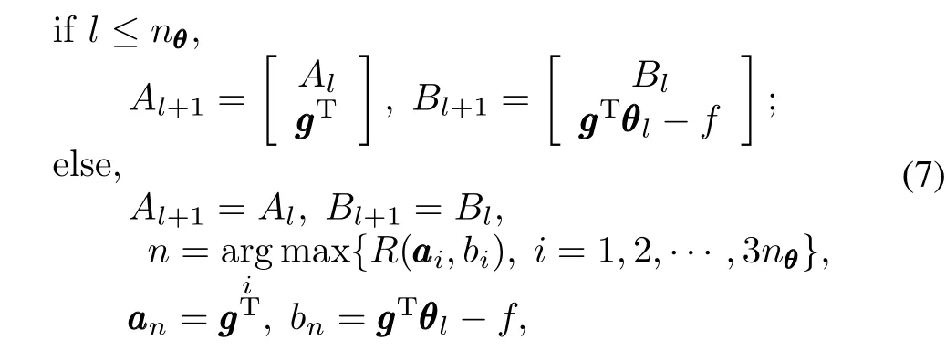
where aaanis the n th row vector of Al+1,and bnis the n th element of Bl+1.In this paper,we limit the total number of inequalities to be 3nθ.
The convergence of the algorithm is guaranteed by the characteristic of the MVE cutting plane method.A theoretical upper bound for the number of outer iterations of the MVE-based SE method,suggested in[18],is also applicable to Algorithm 1,despite its conservativeness.For details about cutting plane methods,readers can refer to[19].If Assumption 1 is notsatisfied,there would be otherwise two specialcases. First,if the primal SCPNproblem(2)is unfeasible,the algorithm will not output any feasible results after proceeding for a large quantity of cycles,even if the number of iterations reaches its upper bound.Second,ifΘ1does not contain the optimaθ?,which is possibly encountered in practice as the initial hypercube may fail to satisfy Assumption 1,the algorithm just finds a sub-optimal solution withinΘ1.
Given an SCPNproblem,Algorithm 1 proceeds in a deterministic framework,although the underlying interpretation is in a probabilistic sense.Different from SE methods,the scenarios used for test are prepared in advance.However,for Algorithm 1,it is still cumbersome to test all the N scenarios in every inner iteration,because the quantity N depends on the dimension of the optimization parameter(see(3)),usually being a large number,larger than that used in SE methods. Consequently,Algorithm 1 has little advantage over the SE methods in respect of algorithm's total execution time.
The basic idea to amend Algorithm 1 is to reduce the numberofscenarios consumed in each innerloop.One natural way is to randomly batch the N scenarios for verification;the underlying idea is thatsuccessive demonstrations of feasibility for the randomly-sampled batches will steadily enhance our confidence on the solution's feasibility for allthe N scenarios. To illustrate the rationale of this idea,we presentthe following theorem.
Theorem 2.Suppose we have to inspect a set of N scenarios.A k-length subset randomly sampled from the N scenarios,called a k-sample batch,is defined to be“good”if and only if the solution is verified to be feasible for all the k scenarios.Then,if m successive k-sample batches have been verified to be good,ourconfidence thatthe solution is feasible for all the N scenarios,denoted by

Proof.For a given solution,letλbe the chance of a scenario to be good,then in a k-sample batch,the number of good scenarios,denoted by“x”,obeys the binomial distribution, i.e.,

where l(x|λ)is a likelihood function.If x = k,(9)is simplified as l(k|λ)=λk.
Then for m successive good k-sample batches that are i.i.d, the likelihood function can be written as

In the Bayesian sense,the posteriorprobability ofλis given by

where g(λ)isλ's prior distribution.For a given N-length set of scenarios,λis a discrete stochastic variable that can be assigned(N+1)values:0,1/N,2/N,···,1.Once a good k-sample batch has been obtained,it is definitely known that λ≥k/N.And further,from a Bayesian point of view,if we have no preference aboutλ's evaluation in interval[k/N,1], it is most reasonable to assumeλto be uniformly distributed in this interval.So g(λ)is given as

Inserting(10)and(12)into(11),the confidence thatλ equals to 1 is then obtained as

Theorem 2 indicates the number of times we have to repeat for sampling inspections if k andηare determined in advance. It then inspires Algorithm 2,for which we just give the iteration part below,as the rest of Algorithm 2 is similar to Algorithm 1.
Algorithm 2.
Iterations:
1)Randomly pick K samples from the set of N scenarios, and perform oracle on this subset.
If?(θl,δ(k))≤0 for all k∈{1,2,···,K}
If Do Batch Check/=1,set
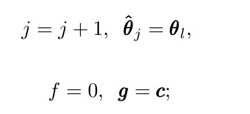
else set f cnt=f cnt+1, θl=θl?1,and go to step 3);
else set f=?(θl,θ(k)),ggg=?θ?(θl,δ(k)),f cnt=0.
2)Update.Add a new cutting plane to Placcording to(7), find the MVE El+1in polytope:


3)Stopping rule.
If f cnt>M,the algorithm stops,
else set l=l+1,and go to step 1).
In the algorithm,N,K and M respectively stand for the total amount of scenarios generated by the SCP problem,the number of scenarios comprising one batch and the number of successive good batches.
Remark 1.For Algorithm 2,at the beginning,everything goes the same way as in Algorithm 1 except the number of scenarios used for feasibility verification,until the objective function cccTθ's descending rate reaches a prefixed threshold τ.Then the algorithm stops improving cccTθ,and tries to find a solution that is able to pass successive verifications on M randomly-picked K-sample batches.
Remark 2.Only the last one of the output set{?θj}is the solution we want,and we recommend a complete feasibility verification ofthis solution on allthe N scenarios.Fortunately, if we have set a high confidence,e.g.,η=0.95,the last one is almost always the“right”one.
Remark 3.The above batch algorithm is designed forrobust optimization problems,and a slight modification to the algorithm will fit it for robust feasibility problems,while merely removing the parts aboutobjective function improvementaway from the iteration process.
III.ROBUST OUTPUT-FEEDBACK CONTROL OF LPV SYSTEM USING ISA
A.Preliminary on Robust LPV Control
Given two compact sets P?RnρandΔ?Rnδ,consider an uncertain LPV systemΣP,Δ,i.e.,


In this paper,we are concerned with the induced L2-norm performance of closed-loop LPV system(13)and(14),which is defined as

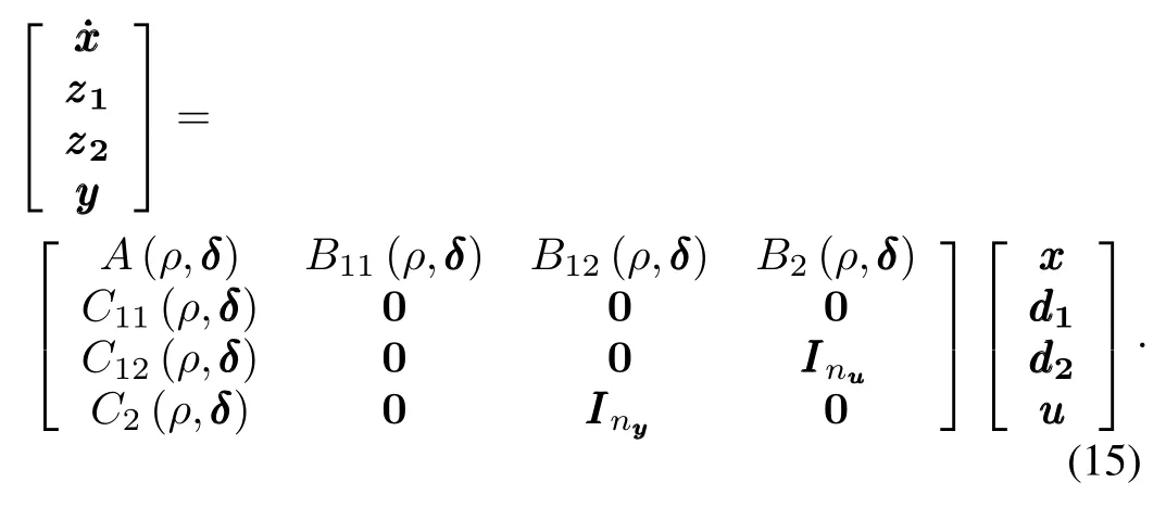
where FPdenotes the setofallpiecewise continuous functions mapping time t into P with a finite number of discontinuities in any interval[20].Following the loop-shifting techniques[21], it is possible to transform any general LPV plant as in(13) to a simplified form PSP,Δ,written as(15),through normpreserving transformations on zzz/ddd and invertible transformations on yyy/uuu:
B.Induced L2-norm Control of LPV System with Uncertainty
For the L2-norm robust control of an LPV system in the presence of model uncertainty,we give a sufficient condition as follows.
Theorem 3.Given the uncertain LPV system PSP,Δ,and a controller KP,the closed-loop system is guaranteed to have an L2-norm performance levelγ>0 if there existtwo symmetric matrices X>0 and Y>0,such thatforallρ∈P andδ∈Δ, the following LMIs hold:

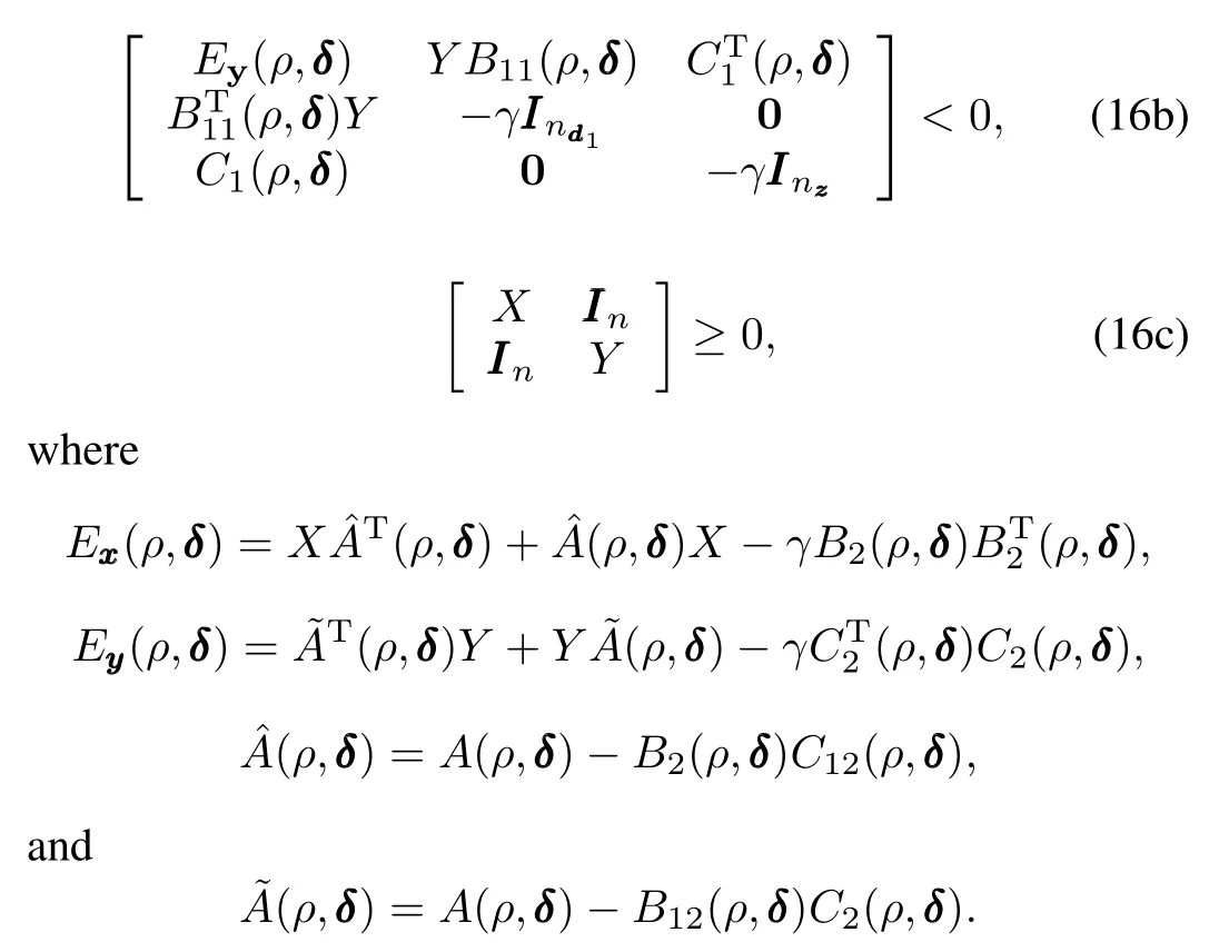
The theorem can be easily proved by directly applying Wu's theorem(see[20],Theorem 3.3.1)on parameter dependent output-feedback controller synthesis,so long as we treat uncertain parameterδthe same way as scheduling parameter ρ,and use the single quadratic Lyapunov function(SQLF) as a degraded form of the parameter-dependent Lyapunov function(PDLF).Once such X and Y are found,we can then construct the robust output-feedback LPV controller based on the nominal state-space matrices.Defi ne[20]
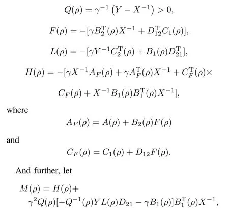
then the n-order strictly proper controller KPachieving γ-performance is presented as
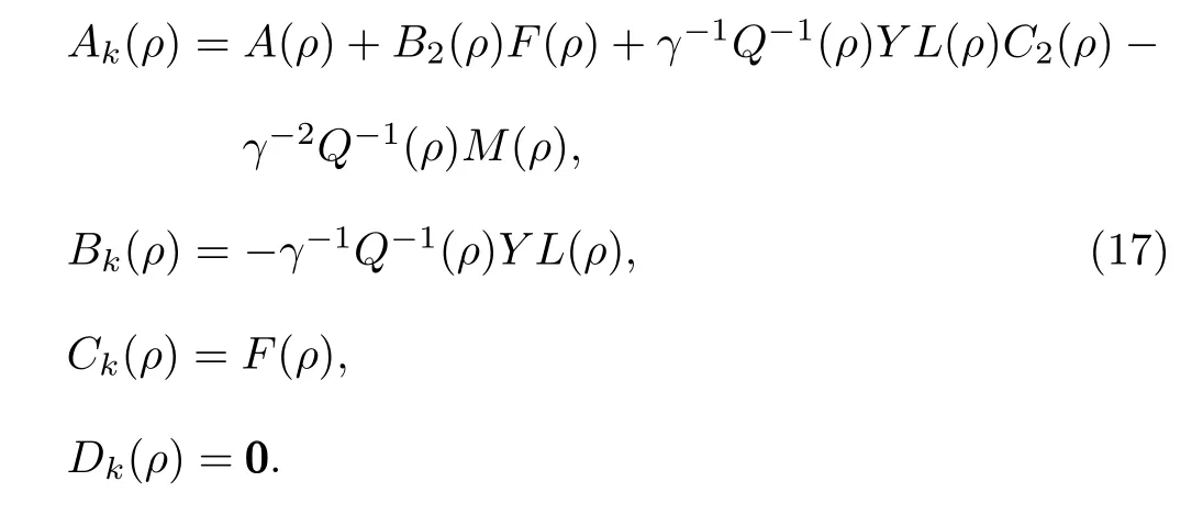
The RCP problem associated with Theorem 3 can be expressed as

whereθdenotes the vector form of the tuple{X,Y,γ}, and Fi(θ,ρ,δ)< 0 represents the LMI constraints arising from Theorem 3.Note that while bothρandδenter the RCP problem in the same manner,they act differently on the system;ρenters the control law as a scheduling parameter, whileδis treated as parameter perturbation whose adverse impactshould be restrained by the controllaw.Therefore,(18) is indeed a robust optimal LPV control problem,taking both demands of gain scheduling and robustness into account.
C.Computational Issues for Applying ISA
To make the ISA algorithms applicable to problem(18), firstly it is necessary to define an equivalent scalar function as well as the associated sub-gradient.Let

where?Fiand ?Fi's dependence onθ,ρandδis omitted for brevity.Then a scalar feasibility indicator function[22]is adopted.Define

where?F+denotes the projection of matrix?F onto the cone of positive semidefinite matrices,and the subscript“fro”denotes the Frobenius norm that we adopt in this paper.It is easy to verify that?(θ,ρ,δ)>0 if and only if?F(θ,ρ,δ)≤0 does not hold,and it is zero,otherwise.Define

Then,the sub-gradient of?(θ,δ)is given as

Then we cope with the parameter dependency problem. Note that?(θ,ρ,δ)≤0(?(θ,ρ,δ)=0 in our case)must hold for allρ∈P.To handle the LMI's dependence onρ, a so-called gridding technique is commonly used[1,23].After L gridding points are selected,i.e.,and scenarios ofδare collected,problem(18)is further approximated as

which has totally L×N constraints.
In this paper,we use a different way to deal with the scheduling parameter,that we cast it as a role of the scenario, generating random samples rather than making grids upon it.This means the scheduling parameters act like uncertainty parameters during the computation,which can be easily understood by observing thatρandδenter problem(18)in thesame manner.So problem(18)is finally translated into the following scenario design problem thatcan be solved by ISA:

The benefit of doing so is obvious that randomly sampling scheduling parameter does not increase the sample size of scenarios,while greatly reducing the number of LMI constraints for each scenario,compared to the gridding approach. And if the solution of(19)exists,it is supposed to be better generalized to allρ∈ P than that of using the gridding approach,as it has experienced more instances ofρ.
IV.APPLICATION TO THE CONTROL OF A SMALL HELICOPTER
A.Model Setup
In this section,the ISA proposed in the above section is applied to design an LPV longitudinal controller of a small helicopter for its cruise flight.We employ a Hirobo 90-class model scale helicopter,shown in Fig.1,as the testbed of our design method.A small helicopter is accurately modeled by the fuselage's 6-DOF rigid body model augmented with the first-order main rotor and stabilizer bar's flapping dynamics, whose complete modeldescription includes 13 states:3 linear velocity components in body-axis(u,v,w),3 angular rates (p,q,r),3 Euler angles(φ,θ,?),2 flapping angles of main rotor's tip-path-plane(TPP)(a1,b1)and 2 flapping angles of Bell-Hiller bar's TPP(c,d).A minimum complexity nonlinear model[24]is used both for linear modelextraction and simulation verification.Earlier work on modeling a small helicopter with stabilizer bar[25]showed thatthe main rotor and stabilizer bar's flapping dynamics could be lumped and modeled just by main rotor's 2-order TPP flapping dynamics,with the stabilizer bar's effect counted into main rotor's equivalent flapping time constant.So for longitudinalmotion,the state vector is defined to be[u a1w q θ]T,where u is the body axis forward speed,a1is the longitudinal flapping angle,w is the vertical speed,q is the pitch rate andθis the pitch angle.
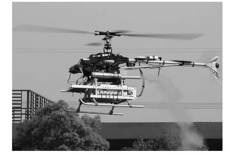
Fig.1. The equipped 90-class model helicopter in flight.
In order to describe the flight dynamics,many physical parameters need to be evaluated,some of which are related to aerodynamics,and rotor flapping are hard to be determined, as listed in Table I.
The listed items are the uncertain parameters we care about for controller design,whose nominalvalues are determined by citing the parameter data of an X-Cell 60-class helicopter[25], and we assume they are uniformly distributed around the nominal values.
The model dynamically varies depending on the advanced ratioμ,defined byμ=u/?R,where?and R are main rotor's revolution,speed and radius,respectively.It is reasonable to select u to be the scheduling parameter,i.e.,ρ=u,as?is usually kept constant by an independent engine controller during the flight.The flight envelope of interest covers the speed regime of 0~25 m/s,so the scheduling parameterρis assumed to be uniformly distributed in this interval.
Following the trim and linearization procedures,the helicopters'longitudinal LPV model can be extracted from its nonlinear simulation model,expressed as(20)in the next page,whereδlonandδcolare longitudinal cyclic input,and collective input,respectively;θeandφeare trimmed angles; X,D,Z,M are the stability derivatives and K is the control derivative;and y denotes the output vector.
B.Controller Design
Similarto the synthesis procedures for LTIsystems,weighting functions are defined here to characterize the overall closed-loop performance.The open-loop interconnection of the corresponding weighted system is shown in Fig.2,where
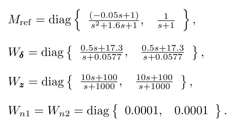
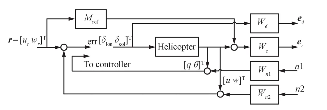
Fig.2. Weighted open loop interconnection of helicopter plant.
From the interconnection shown in Fig.2,it is easy to construct a 12-order augmented open-loop LPV model of the form(13)for the longitudinal dynamics.The corresponding SCP has 157 design variables.To get an initial guess of the design variables,standard SA is implemented on 1 000 scenarios using YALMIP[26]under Matlab environment,which nearly uses up the computational capacity of a personal computerequipped with 2 GB memory.The calculated optimal performance level is 2.09,and the initial guess ofγis set to be 6.0,allowing some gap above the calculated value. The initialhypercube constraints,centered on the initialguess mentioned above,are chosen to be large enough to guarantee the confidence that the optima are included in the hypercube, whose volume is about 2.62×10365.
We setτ=0.07,ε=0.05,andβ=10?5to execute the proposed two ISA algorithms.According to(3),6 742 scenarios are created.For Algorithm 2,we selectη=0.95,and K=400,and then using(8),the repeattimes ofsampling inspection,M,is set to be 51.For comparison,we also implementin the same settings,the SE algorithm based on the MVE cutting-plane method,which is proposed by Wada etal.[18]and regarded as the most sophisticated framework among current SE methods.All the algorithms are implemented on a personal computer with 2.26 GHz CPU and 2 GB memory. Table IIshows the process information ofthe three algorithms.

TABLE I UNCERTAIN PARAMETERS OF A SMALL HELICOPTER AND THEIR DISTRIBUTIONS

In Table II,the execution time(the 4th column)of the algorithms involves both the time spent on the iterations and the time to generate enough scenarios for the algorithm;the latter is particularly listed in the brackets to facilitate the comparison.As observed from the table,Algorithm 1 is the least efficient in the respect of execution time;the scenarios consumed by Wada's algorithm are nearly 3 times that of Algorithms 1 and 2,thus making itrather sluggish;the batch algorithm(Algorithm 2)spentjust 45%of the time taken by Wada's algorithm.
C.Simulation Results
We apply Monte Carlo approach to verify the robust feasibility of the solutions obtained from different algorithms. Firstly,we estimate the empirical probability of robust feasibility for both nominal solution and the solutions by the three algorithms mentioned above,by checking whether the LMIs (16 a)~(16 c)(or?(δ,ρ,θ)≤0)hold for each test scenario. Secondly,to verify the actualclosed-loop robustness,we adopt the closed-loop LMI formula[20]that conditions theγ-level L2-norm performance,given by
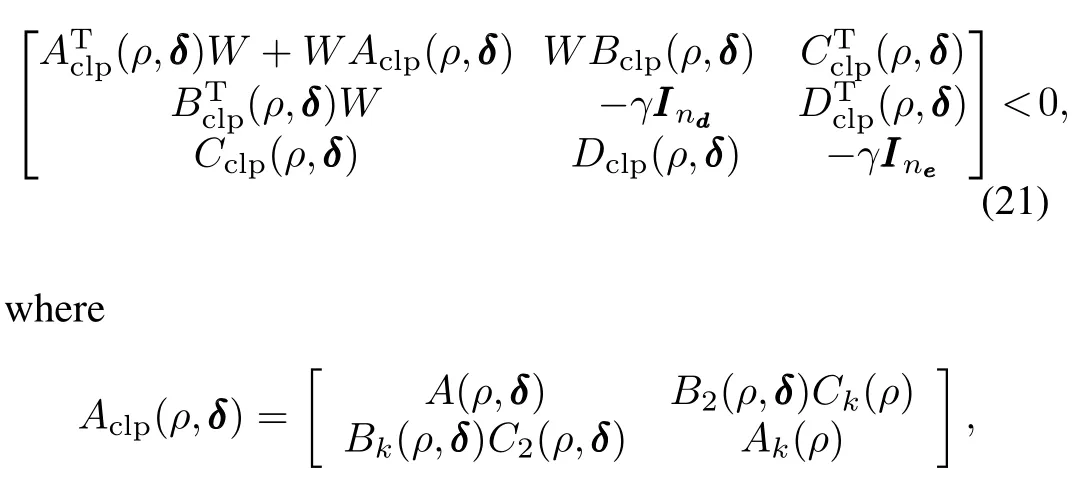
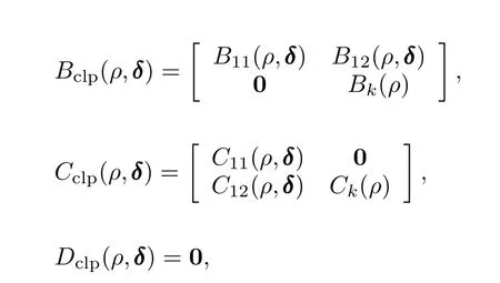
and W is the matrix associated with the Lyapunov function of the closed-loop system,defined here by

Ten thousand scenarios are generated for the verifications, and the results are shown in Table III.Forcomparison purpose, we also putinto the table the results obtained from other three algorithms:LPV control(LPV-C)on nominal plant,SA on 1 000 scenarios(whose solution is used as the initial guess of the iterative algorithms),and Wada's algorithm.
From Table III,it seems that the robustness improvement is encouraging after performing the first kind of verification,as the empirical estimates of probabilistic robust feasibility for both Algorithms 1 and 2 are much better than their theoretical bounds.However,the results of closed-loop LMI verification are a bit disappointing.Recall that in order to make the controller implementable,we constructitbased on the nominal plant,see(17)where we use A(ρ)rather than A(ρ,δ).As discussed in Section III,bothρandδactin the same way from a pure mathematical point of view,and in the general SQLF settings,A(·)should depend on bothρandδ.So neglecting its dependence on the uncertaintyδresults in a loss ofrobustness. But from a practical point of view,things are still acceptable. Similar results were reported in[23],but the performance degradation of ours is remarkably smaller.
Finally,the closed-loop performance of robust LPV controller constructed using the solution of Algorithm 2 is verified through simulations on helicopter's nonlinear model.To construct the controller as formulated in(17),nominal LPV matrices A(ρ)and B(ρ)are approximated by polynomialmatrices driven byρ.We exert step-like reference signal to either forward or verticalchannels respectively,while keeping the other at zero state.Ten uncertain nonlinear models are used for the verification,and the results are shown in Figs.3 and 4,where the dashed lines representthe desired responses (outputofthe reference model)and the solid lines representthe actualresponses.Note thatthe nominal LPV controller cannot pass the closed-loop feasibility verification for any scenario candidate,as shown in Table III,so there is no need to verify it on the nonlinear model again.

TABLE II PROCESS INFORMATION OF DIFFERENT ALGORITHMS

TABLE III FEASIBILITY VERIFICATION RESULTS OF DIFFERENT ALGORITHMS
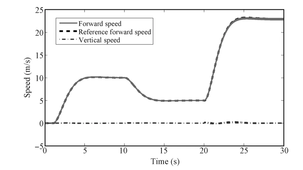
Fig.3. Forward and vertical speed responses to step-like excitation on the forward speed channel.
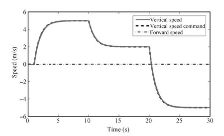
Fig.4. Forward and vertical speed responses to step-like excitation on the vertical speed channel.
From Figs.3 and 4 seen that in the presence of model perturbations,the closed-loop system tracks reference model outputs very well.This means that governed by the LPV controller,the system consistently presents a second-order closed-loop characteristic specified by the reference modelin a wide speed range(0~23 m/s),which is quite desirable for the high-layer motion planning design.Itis further observed from Fig.3 that the variation of vertical speed is kept very small during the high-speed forward flight,which means that the longitudinal phugoid mode is eliminated,demonstrating that the decoupling performance of the controller is satisfactory.
D.Discussion
For a complex system like a small helicopter,neither trim nor linearization procedures are simple,as seen from Table Iit takes more than 1 s to create a scenario.In this situation,those SE algorithms are too time-consuming.The proposed batch algorithm(Algorithm 2)adopts both advantages of Algorithm 1 and SE algorithms,i.e.,it consumes the same amount of scenarios in all as the former,and queries as many as the latter for feasibility verifications.
Numerical stability is a problem of optimization algorithms using cutting-plane techniques.For the controller design of a smallhelicopter's longitudinalmotion,a 157-dimensionaloptimization problem,numericalstability would gradually deteriorate,i.e.,the condition numbers of the matrices generated from the algorithm become much larger,as the cutting-plane-based algorithm proceeds.The algorithm might stop unexpectedly with fatal errors,if we cancel the constraint pruning codes. The aforementioned heuristic logic for removing redundant constraints can effectively improve the numerical stability as no fatal error occurs once the logic works.However,the curse of dimension is still a problem that we cannot thoroughly circumvent.For SCP problems oflarger-scale,e.g.,largerthan 157-dimensions,a more elaborate constraintpruning technique would be necessary.
V.CONCLUSIONS
In this paper,we have presented iterative algorithms for the SA.For the robustcontrolof a complex LPV system which is time-costly to create through linearization,the proposed batch algorithm has been shown to be more efficientthan the popular SE methods.In the robust LPV control context,we have also proposed to cope with parameter dependency using the randomization technique identically on both uncertainty andscheduling parameters,and to prune the redundant constraints using a heuristic logic based on relevance ratio ranking. All these techniques together comprise a complete method, which has been applied to design robust LPV controller for small helicopter's cruise flight.Multiple uncertain physical parameters have been considered.Simulation studies have been provided to demonstrate its effectiveness.
REFERENCES
[1]Rugh WJ,Shamma JS.Research on gain scheduling.Automatica,2000, 36(10):1401?1425
[2]Helmersson A.μ-synthesis and LFT gain scheduling with realuncertainties.International Journal of Robust and Nonlinear Control,1988,8(7): 631?642
[3]Helmerson A.Application of real-μgain scheduling.In:Proceedings of the 35th IEEE Conference on Decision and Control,Kobe,Japan:IEEE, 1996.1666?1671
[4]Apkarian P,Adams R J.Advanced gain-scheduling techniques for uncertain systems.IEEE Transactions on Control System Technology, 1998,6(1):21?32
[5]Aouani N,Salhi S,Garcia G,Ksouri M.Robust control analysis and synthesis for LPV systems under affine uncertainty structure.In:Proceedings of the 6th International Multi-conference on Systems,Signals and Devices,Djerba,Tunisia:IEEE,2009.187?191
[6]Veenman J,Scherer C W.On robustLPV controllersynthesis:a dynamic integralquadratic constraintbased approach.In:Proceedings ofthe 49th IEEE Conference on Decision and Control,Atlanta,USA:IEEE,2010. 591?596
[7]Calafiore G,Dabbene F,Tempo R.A survey of randomized algorithms for control synthesis and performance verification.Journal of Complexity,2007,23(3):301?316
[8]Kanev S,De Schutter B,Verhaegen M.An ellipsoid algorithm for probabilistic robust controller design.System&Control Letters,2003, 49(5):365?375
[9]Calafiore G,Dabbene F.A probabilistic analytic center cutting plane method for feasibility of uncertain LMIs.Automatica,2007,43(12): 2022?2033
[10]Calafiore G,Dabbene F,Tempo R.Research on probabilistic methods for control system design.Automatica,2011,47(7):1279?1293
[11]Calafiore G,CampiMC.The scenario approach to robustcontroldesign. IEEE Transactions on Automatic Control,2006,51(5):742?753
[12]Calafiore G,Fagiano L.Stochastic model predictive control of LPV systems via scenario optimization,Automatica,2013,49(6):1861?1866
[13]Campi M C,Garatti S,Prandini M.The scenario approach for systems and control design.Annual Reviewsin Control,2009,33(2):149?157
[14]Wang X,Lu G,Zhong Y.Robust H∞attitude controlofa laboratory helicopter.Roboticsand Autonomous Systems,2013,61(12):1247?1257
[15]Liu C,Chen W,Andrews J.Tracking control of small-scale helicopters using explicit nonlinear MPC augmented with disturbance observers. Control Engineering Practice,2012,20(3):258?268
[16]Cai G,Chen B M,Dong X,Lee T H.Design and implementation of a robust and nonlinear flight control system for an unmanned helicopter. Mechatronics,2011,21(5):803?820
[17]Simpl′?cio P,Pavel M D,van Kampen E,Chu Q P.An acceleration measurements-based approach for helicopter nonlinear flight control using incremental nonlinear dynamic inversion.Control Engineering Practice,2013,21(8):1065?1077
[18]Wada T,Fujisaki Y.Sequential randomization algorithms:a probabilistic cutting plane technique based on maximum volume ellipsoid center.In:Proceedings of the 2010 IEEE International Symposium on Computer-Aided ControlSystem Design,Yokohama,Japan:IEEE,2010. 1533?1538
[19]Localization methods[Online],available:http://www.stanford.edu/ class/ee392o,September 1,2011
[20]Wu F.Controlof Linear Parameter Varying Systems[Ph.D.dissertation], University of California at Berkeley,USA,1995
[21]Safonov M,Limbeer D,Chiang R.Simplifying the H∞theory via loop shifting,matrix pencil,and descriptor concepts.International Journal of Control,1989,50(6):2467?2488
[22]Calafiore G,Polyak B T.Stochastic algorithms for exact and approximate feasibility of robust LMIs.IEEE Transactions on Automatic Control,2001,46(11):1755?1759
[23]Lu B,Wu F.Probabilistic robust linear parameter-varying control of an F-16 aircraft.AIAA Journal of Guidance,Control,and Dynamics,2006, 29(6):1454?1459
[24]Heffley R K,Mnich M A.Minimum-complexity Helicopter Simulation Math Model.Technical Report 19880020435,NASA,USA,1988
[25]Gavrilets V.Autonomous Aerobatic Maneuvering of Miniature Helicopters[Ph.D.dissertation],Massachusetts Institute of Technology, 2003.
[26]L¨ofberg J.YALMIP:A toolbox for modeling and optimization in MATLAB.In:Proceedings of the 2004 IEEE International Symposium on Computer Aided Control Systems Design,Taipei,China:IEEE,2004. 284?289

Zhou Fang Associate professor in the School of Aeronautics and Astronautics,Zhejiang University, China.He received his Ph.D.degree from the Department of Control Science and Engineering, Zhejiang University in 2008.His research interests include navigation,guidance and control of UAVs and advanced learning controlmethods.Corresponding author of this paper.
Hua Tian Ph.D.candidate in the Department of Control Science and Engineering,Zhejiang University,China.Her research interests include modeling and control of UAVs.

Ping Li Professor of both the Schoolof Aeronautics and Astronautics and the Departmentof ControlScience and Engineering,Zhejiang University,China. His research interests include process control,UAV projects and intelligenttransportation systems.
RC has
lots of attentions in control community since late 1990s.Various algorithms and their applications are documented,which are classified into three main methodologies by Calafiore etal.[7]:the approach based on the statistical learning theory,the sequential approximation methods based on gradientiterations orstochastic ellipsoid(SE)iterations,and the scenario approach(SA).SE algorithms[8?10]proceed in an iterative scheme,online generating scenarios for oracle,and the sample size per iteration is independent of both the number of uncertainty parameters and the number of the design variables.So SE approaches seem to perform quite efficiently,and have been the mostpopular PRC methods currently.However,for an SE algorithm,the total amount of scenarios consumed by all the iterations is very large, even much larger than that of SA.So for controller synthesis problems of LPV systems,whose linearization procedure may need a great deal of calculation,SE methods might be too time-consuming.
Manuscriptreceived October 10,2013;accepted April11,2014.This work was supported by National Natural Science Foundation of China(61004066). Recommended by Associate Editor Bin Xian
:Zhou Fang,Hua Tian,Ping Li.Probabilistic robust linear parameter-varying control of a small helicopter using iterative scenario approach.IEEE/CAA Journal of Automatica Sinica,2015,2(1):85?93
Zhou Fang is with the School of Aeronautics and Astronautics,Zhejiang University,Hangzhou 310027,China(e-mail:zfang@zju.edu.cn).
Hua Tian is with the Departmentof Control Science and Engineering,Zhejiang University,Hangzhou 310027,China(e-mail:htian@iipc.zju.edu.cn).
Ping Li is with the School of Aeronautics and Astronautics,Zhejiang University,Hangzhou 310027,China and Department of Control Science and Engineering,Zhejiang University,Hangzhou 310027,China(e-mail: pli@iipc.zju.edu.cn).
 IEEE/CAA Journal of Automatica Sinica2015年1期
- IEEE/CAA Journal of Automatica Sinica的其它文章
- Decoupling Trajectory Tracking for Gliding Reentry Vehicles
- Autonomous Landing of Small Unmanned Aerial Rotorcraft Based on Monocular Vision in GPS-denied Area
- Guest Editorial for Special Issue on Autonomous Control of Unmanned Aerial Vehicles
- A Predator-prey Particle Swarm Optimization Approach to Multiple UCAV Air Combat Modeled by Dynamic Game Theory
- Adaptive Backstepping Tracking Control of a 6-DOF Unmanned Helicopter
- Continuous Sliding Mode Controller with Disturbance Observer for Hypersonic Vehicles
