Three-dimensional prediction of reservoir water temperature by the lattice Boltzmann method: Validation*
DIAO Wei (刁偉), CHENG Yong-guang (程永光), ZHANG Chun-ze (張春澤), WU Jia-yang (吳家陽)
State Key Laboratory of Water Resources and Hydropower Engineering Science, Wuhan University, Wuhan 430072, China, E-mail: wdiao@whu.edu.cn
Introduction
Quite a number of high dams and large reservoirs were built in China. By 2013, more than 150 dams higher than 100 m were erected and over 750 large reservoirs built, with a total water capacity of 7×10¹¹cubic meters. These reservoirs play important roles in the flood control, the power generation, the navigation,the irrigation, and the tourism. In these scenarios, the thermal stratification in high-dam reservoirs is an important issue. The temperature of a large deep reservoir usually varies by more than 10oC, and the temperature in the middle and bottom regions remain at the level of about 12oC-13oC. The stratification may cause physical and chemical changes in the properties of the water, affect the ecological balance of the environment, hamper the growth of irrigated plants, and even have impacts on the normal life of local residents[1]. Therefore, an effective and efficient simulation and prediction of the reservoir water temperature is important for promoting a harmonious hydraulic development and an ecological protection.
Currently, the basic methods for studying the water temperature distribution in reservoirs include the empirical/analogical methods[1,2], the physical model tests[3,4], and the numerical models[5,6]. Of these,the empirical/analogical method can provide only an approximate 1-D vertical distribution, and the physical model tests are costly, time consuming, and restrictive in the assessment of physical phenomena. Only the numerical method can strike a balance between accuracy, efficiency, economy, and applicability, which makes it the most suitable approach for predicting the temperature distribution. Of the numerical methods available, the 3-D model is the most powerful and promising because it can provide detailed temporal and spatial patterns of temperature and flow, although the 1-D and 2-D methods are still dominant in use[7].
The lattice Boltzmann method (LBM), based on the kinetic theory, is a newly developed computing technique for simulating complex fluid flows. It hasbeen applied successfully to the simulations of the large-scale flow, the multi-phase flow, the multi-component flow, the porous media flow, and other flows.Because of its many advantages, including its simple algorithm, the intrinsic parallelism, and the simple implementation of boundary conditions, the LBM has shown greater development prospects than the traditional numerical methods for fluid mechanics[8]. The LBM models for thermal fluid flows can be classified in three categories: the multi-speed approach[9], the multi-distribution function approach[10], and the combined approach[11]. These thermal models were used successfully to simulate practical heat transfer problems[12], but their applications to the predictions of the water temperature distributions in reservoirs or lakes are few.
This paper presents simulations of the process of the water temperature variation in a model reservoir,in a benchmark test by the US Army Corps of Engineers Waterways Experiment Station[4]. An LBM model, based on the large-eddy simulation for thermal buoyancy flows, is adopted to simulate and analyze the temporal and spatial variations of the reservoir water temperature, to validate the method, and to analyze the mechanism of the gravity sinking current.
1. Computational models for reservoir water temperature
1.1 Double distribution function LBM model based on Boussinesq assumption
The reservoir water is normally considered as incompressible, with the density, the viscosity, and the thermal diffusivity being also assumed to be constant except for the buoyant body force. Therefore, the governing equations for the model of the reservoir water flow can be expressed with the Boussinesq assumption[13]as:
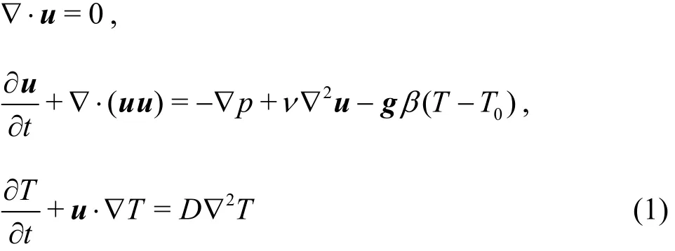
wherepis the pressure,Dis the diffusivity,νis the viscosity,βis the thermal expansion coefficient,andT0is the average temperature.
To solve Eq.(1), the double-distribution-functionbased LBM (DDF-LBM) model may be used. The DDF-LBM, first developed by Bartoloni in 1993[14],models the velocity and temperature fields by two respective distribution functions and the two fields are coupled by a body forcing term in the flow field. Here,based on the improved 2-D DDF-LBM of Guo at al.[10], we extend the model to the 3-D form using the D3Q19 model for the velocity field simulation and the D3Q6 model for the temperature field simulation. The LBM equations for these two fields may be expressed as follows:
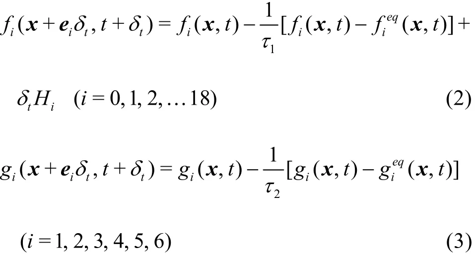
in whichfiandgiare the distribution functions for the water flow and the temperature field, respectively,andare the corresponding equilibrium distribution functions,τ1andτ2are the relaxation factors, andHiis the buoyant forcing term.
The equilibrium distribution functions can be expressed as:
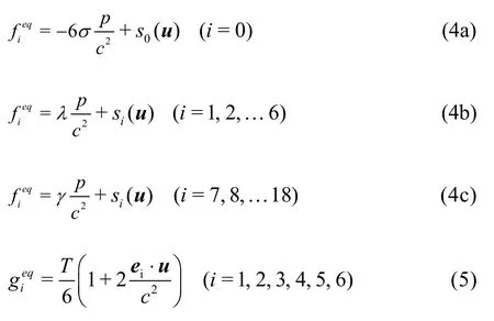
whereuis the velocity vector,Tis the temperature,σ,λandγare the parameters satisfyingλ+2γ=σandλ+2γ=1/3, and chosen as 1/3, 1/6, and 1/12 in this work, respectively.si(u) can be expressed as a function of the macroscopic velocityuand the discrete velocityei.

whereiωis the weight coefficient in the D3Q19 model, andcsis the speed of sound.
The macroscopic velocityu, the pressurep,and the temperatureTare expressed in the moments of the distribution functions as

The viscosityν, the diffusivityD, and the Prandtl numberPrare determined by

The coupling of the velocity field with the temperature field is realized by attaching an additional forcing termHito Eq.(2). The introduction of this forcing term is essential for the accuracy and the stability of the coupling scheme. We adopt the newly proposed approach by Cheng and Li[14]because it has been verified to be stable and accurate for treating non-uniform, unsteady forcing and source terms. According to the Ref.[15], the forcing termHican be expressed as

in which

whereAis the source term in the continuity equation andBis the forcing term in the momentum equation.Considering Eq.(1), we setA=0 andB=-gβ(TT0).
It should be noted that using the D3Q6 model for the 3-D temperature field can save the computer memory usage and increase the speed of the calculation.However, when treating complex boundary problems,the number of discrete particle velocities should be increased to retain good accuracy and stability.
1.2 Large eddy simulation based on LBM
When a subgrid-scale model is used in the large eddy simulation, the physical quantities of the fluid flow can be divided into two parts: the large-scale and small-scale quantities[16]. Taking′, for example.is the filtered largescale quantities ofφusing the filter functionGandrepresents the small-scale fluctuations being modeled.

in which the distribution functions are all filtered quantities. The relaxation timeis not a constant but is a variable that changes with time and space, which can be calculated by the total viscosity=, whereνandare the molecular and eddy viscosities, respectively. According to the Smagorinsky model[13],can be obtained by=, whereC, Δ andare the Smagorinsky constant, the filter width, and the strain-rate tensor, respectively. The strain-rate tensor can be calculated easily by using the second order moments of the filtered particle distributions[16].
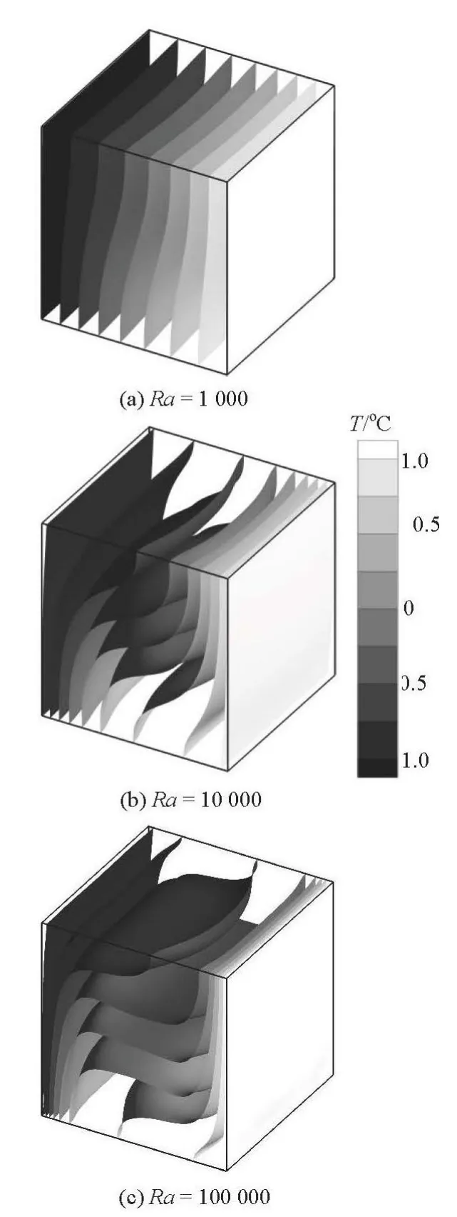
Fig.1 Isothermal surfaces for natural convection in a cubic cavity
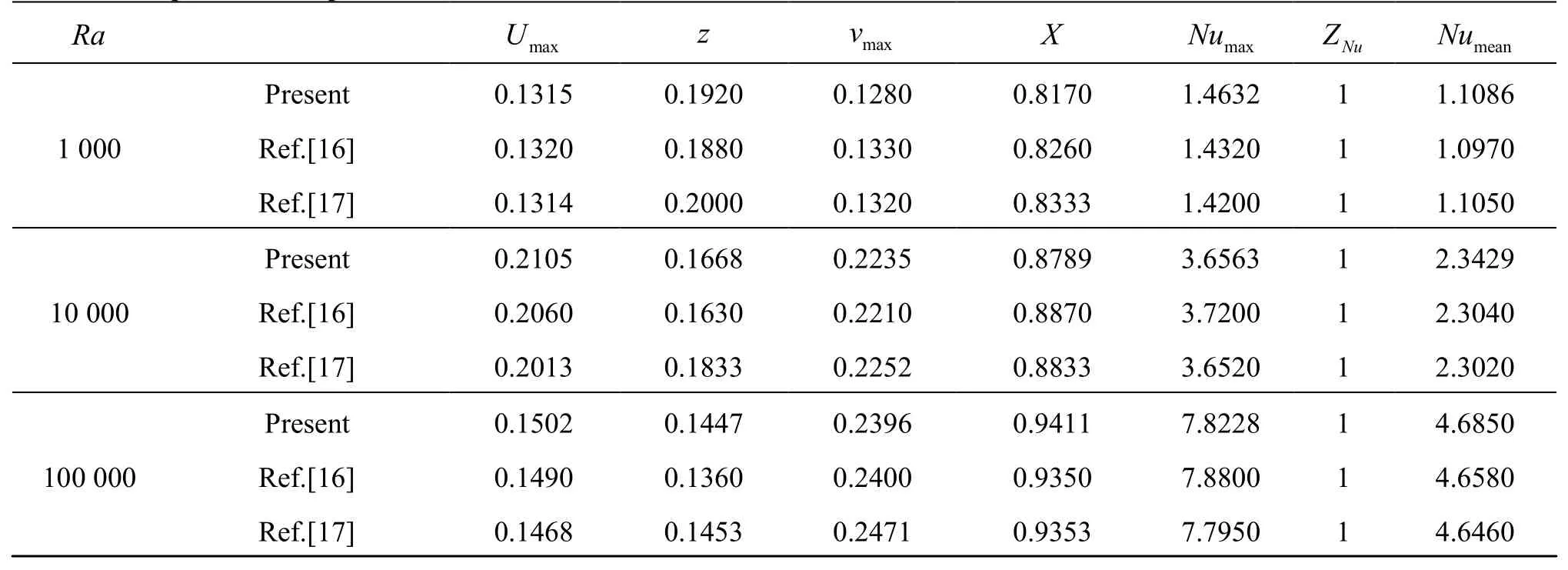
Table 1 Comparison of representative field values
2. Model verification
2.1 Natural convection in a cubic cavity
Initially, the natural convection in a cubic cavity ofL×L×Lis simulated. The hot wall ofTh=1oC is on the right-hand side and the cold wall ofTc=?1oC is on the left[16]. The initial temperature is set asT0=(Th+Tc)/2. The Rayleigh and Prandtl numbers are defined byandPr=ν/D,respectively. A lattice ofNx×Ny×Nz=81× 81× 81 is applied, andPr=0.71 andRa=103, 104, and 105are given.
The simulated isothermal surfaces for the natural convection flows at different Rayleigh numbers are shown in Fig.1.
Table 1 lists some representative results of the flow field in the symmetry plane (y=Ny/2) for comparison with those in the literature[16,17]. These representative results include the maximum horizontal velocityon the vertical mid-line and its correspondingZcoordinate, the maximum vertical velocityon the horizontal mid-line and its correspondingXcoordinate, the maximum Nusselt numbersat the vertical boundary (x=0) and its locationZNu, and the average Nusselt numberTable 1 shows that the results obtained in this paper agree well with those in Ref.[17].
2.2 3-D Rayleigh-Bénardconvection
The Rayleigh-Bénard convection is another benchmark that generates regular flow and temperature patterns in a cavity with a heated bottom and a cooled top.
The initial temperature of the flow isTc=?1oC.The hot wall ofTh=1oC is on the bottom and the cold wall ofTc=?1oC is on the top. The Rayleigh and Prandtl numbers are defined by/(νD) andPr=ν/D, respectively. This simulation is carried out with a lattice ofNx×Ny×Nz=201×201×51, andPr=0.71 andRa=10000 are applied.
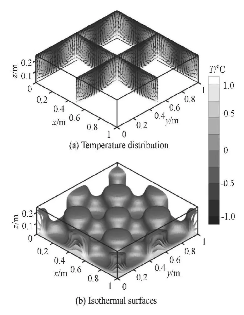
Fig.2 Simulated 3-D Rayleigh-Bénard convection
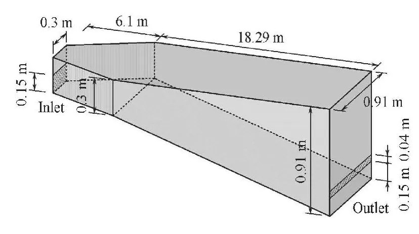
Fig.3 Schematic diagram and dimensions of model reservoir
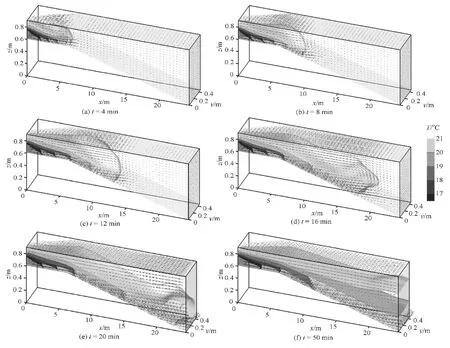
Fig.4 Isothermal surfaces of reservoir water at different times
Figure 2(a) shows the temperature distributions and the velocity vectors of the 3-D Rayleigh-Bénard convection at different planes, includingx=0 and 0.5,y=0 and 0.5, andz=0. The isothermal surfaces where the temperature is above 0oC are shown in Fig.2(b). The good pattern symmetry and the stable cell rotation can be observed in Fig.2, which shows the basic feature of the Rayleigh-Bénard convection and demonstrates the modeling capability of the present model.
3. Temporal and spatial variations of temperature in a reservoir
3.1 Test of gravity sinking current in a model reservoir
The experimental data of the gravity sinking current in a model reservoir, tested by the US Army Corps of Engineers Waterways Experiment Station,are used to validate further the LBM model. As shown in Fig.3, the geometry of the model reservoir can be divided into two parts: a horizontally expanding channel of 6.1 m in length, and 0.3 m in initial depth,which increases linearly from 0.3 m to 0.91 m, and a vertically deepening channel of 18.29 m in length, and 0.91 m in initial width, which increases linearly from 0.3 m to 0.91 m. The inlet, located at the bottom of the left-hand wall, is an orifice of 0.15 m in height. The outlet, located at the right-hand wall, is a narrow rectangular hole of 0.04m in height situated 0.15 m above the bottom. Initially, the reservoir water is stationary with a uniform temperature of 21.44oC. When the test begins, the cold water with a temperature of 16.67oC flows into the reservoir at a rate of 0.00063 m3/s, and the outlet is drained at the same flow rate to maintain a constant water surface level[5].
3.2 Simulation conditions
Considering the geometry and the flow symmetry,only half the flow domain is simulated by the DDFLBM model to reduce the memory requirement and improve the speed. The slip boundary condition and the symmetric boundary condition are imposed at the top and symmetric planes of the reservoir, respectively. A uniform water velocity of 0.014 m/s is imposed at the inlet, while the outflow boundary, by extrapolation, is specified at the outlet. Other boundaries are treated as non-slip walls. For the thermal boundary conditions, the temperatures of 21.44oC and 16.67oC are maintained at the top and the inlet, respectively,and all other boundaries are set as adiabatic. The Prandtl numberPris 7 when the temperature of the water is around 20oC. The kinematic viscosityν=0.003021m2/s and the diffusivityD=0.000431are specified. The simulation is conducted on a 2 440×46×92 lattice.
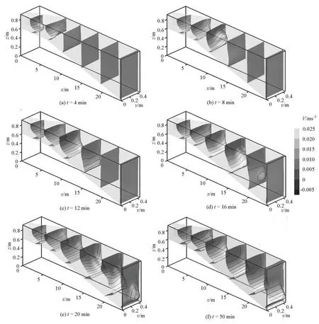
Fig.5 Velocity vectors of reservoir flow at different times
3.3 Temporal and spatial variations of reservoir water temperature
Figure 4 shows the isothermal surfaces of the reservoir water temperature at timet=2 min, 8 min,12 min, 16 min, 20 min and 50 min and Fig.5 shows the velocity field at the corresponding times.
The entire process of the thermal stratification falls into four stages. (1) When the cold water flows as a jet from the inlet into the warmer reservoir, the front,characterized with a large temperature gradient,moves forwards along the bottom, as shown in Fig.4(a). However, no strong vertical convection occurs because of the sinking force from the density difference, although a weak recirculation flow is causedin the upper region, as shown in Fig.5(a). This process may be denoted as the jet penetrating stage. (2) As the cold current front reaches the vertically deepening section of the reservoir, the current accelerates owing to the gravity effect and it moves with transversally nonuniform velocities along the bottom slope, forming a tongue-shaped front, as shown in Fig.4(b). The temperature difference between the cold current and the upper warm water restrains the vertical momentum transfer and generates a sharp vertical velocity gradient, as shown in Fig.5(b). With the further advance of the cold current into the deeper water along the reservoir bottom slope, the current tongue grows thicker and the recirculation region becomes larger, as shown in Fig.4(c) and Fig.5(c). At this moment, the stage of the tongue-like isothermal surface is completed. (3)Subsequently, the temperature within the tongue reduces slowly, while the temperature gradient between the cold current and the warm water remains. The large temperature gradient also restrains the vertical momentum and energy transfers, and causes an obvious thermal stratification of the reservoir water, as shown in Fig.4(d). Corresponding to the temperature distribution, the velocity field also maintains a sharp gradient across the interface of the cold and warm water. The water in the upper region flows in the reverse direction and the water ahead of the tongue flows vertically, forming an expanding recirculation flow region, as shown in Fig.5(d). This is the stage of forming the thermal stratification. (4) When the tongue front of the cold current reaches the right boundary or the dam wall, the stage of forming the horizontal temperature layers begins. In this stage, the cold water begins to accumulate in front of the dam and the isothermal surface of 21oC becomes flat, as shown in Fig.4(e). The recirculation region becomes the longest with the velocity in the front rising along the vertical dam wall, as shown in Fig.5(e). Gradually, the cold water occupies more of the lower space within the reservoir, the isothermal surface of 21oC becomes flat across a broad region, whereas the isothermal surfaces of 18 and 19oC remain parallel with the bottom slope,as shown in Fig.4(e) and Fig.4(f). The entire reservoir is dominated by a recirculation flow, in which the strong cold current gradually expands in the thickness direction as it flows along the bottom slope, while the water in the other region flows in the opposite direction, as shown in Fig.5(e) and Fig.5(f).
During the above processes, the temperature difference between the inflow water and the still water restricts the vertical convection and the turbulent fluctuation. A stable cold sinking current causes the formation and the development of the thermal stratification in the entire reservoir. This strong coupling phenomenon of the velocity and temperature fields indicates that the correct simulation of the turbulent and buoyant flows is an important factor for predicting the thermal stratification of the reservoir water.
The above characteristics of the temperature and the flow agree well with the results calculated by using the Fluent commercial software by Tang et al.[19].
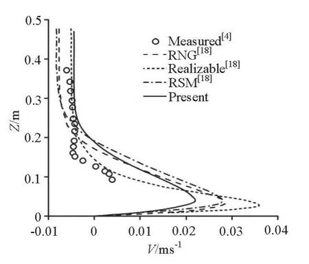
Fig.6 Comparison of velocityuxprofiles at x =11.43m and t =11min on the symmetric plane
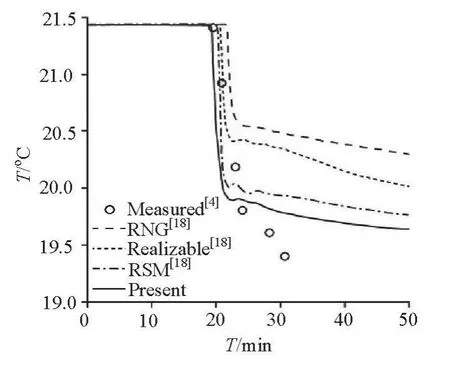
Fig.7 Comparison of the histories of drained water temperature
3.4 Velocity profiles and drained water temperature
Figure 6 compares the velocity profiles along a vertical line 11.43 m from the inlet of the reservoir at the time of 11 min. The RNG, RSM, and Realizable curves are obtained from the Fluent software[19], and the measured data are from the original test[4]. The present results show that the peak velocity of the cold current is about 0.023 m/s and that the peak reversal flow velocity in the upper water is about 0.005 m/s,they are smaller than the measured data and the current thickness is larger than the measured data. This is because the present simulation is performed with a uniform cubic lattice with a grid that is too coarse to reflect properly the sharp velocity gradient of the boundary layer. This can be proved by the comparison of the simulation results on different meshes in the subsection 4.5. On the other hand, no turbulent boundary layer function is applied in the simulation with the subgrid-scale model, which may affect the velocity profiles near the solid boundary. Figure 7 shows the histories of the drained water temperature at the outlet of the reservoir by different methods. Among the four numerical results, those from the present work agreebest with the measured data.
This simulation is run on a PC with 4 cores of 2.66 GHz CPU in MATLAB codes. The number of lattices in this simulation is about 5.5×10⁶, and it takes about 170 h to complete the 50 min process. Obvious speedup may be achieved in the future GPU parallelization.
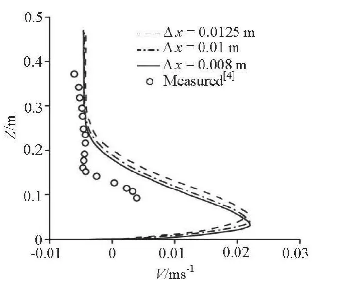
Fig.8 Comparison of profiles of velocity ux atx=11.43m and t=11min on the symmetric plane by different meshes
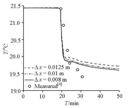
Fig.9 Comparison of the temperature histories of the drained water by different meshes
3.5 Comparison of results by different meshes
To examine the lattice dependence of the solutions, simulations on three different meshes are conducted. Figure 8 shows the profiles of the velocityuxand Fig.9 shows the temperature histories of the drained water by lattice sizes Δx= Δy=0.0125 m, 0.01 m and 0.008 m. It is evident that the results by the coarse lattice of Δx= Δy=0.0125m show larger relative error than those by the fine lattice of Δx= Δy=0.01 m. But the differences of relative errors between the lattice 0.01 m and 0.008 m are not significant. This suggests that the results in the last section are obtained on a convergent grid.
4. Conclusion
A double-distribution-function LBM model is proposed for the 3-D prediction of the reservoir water temperature. This Boussinesq-assumption-based buoyant flow model is verified by two benchmarks: the natural convection in a cubic cavity and the Rayleigh-Bénard convection instability. The temporal and spatial variations of the temperature and the flow in a model reservoir are simulated to validate the method.The general agreement between the measured data and other numerical results demonstrates the accuracy and the efficiency of the present method. The method to treat the turbulent boundary layer and a locally refined grid might be adopted to improve the present model.Implementing the method on GPU chips to improve the simulation efficiency and applying it to flow and temperature predictions of actual reservoirs and lakes will be conducted in the future.
[1] ZHANG Xian-E, ZHOU Xiao-de and ZANG Lin. Discussion on research methods for the water temperature in reservoir[J]. Journal of Water Resources and Water Engineering, 2006, 17(3): 1-4(in Chinese).
[2] ZHANG Shi-jie, PENG Wen-qi. Water temperature structure and influencing factors in Ertan Reservoir[J].Journal of Hydraulic Engineering, 2009, 40(10):1254-1258(in Chinese).
[3] LIU L., LIU D. and JOHNSON D. M. et al. Effects of vertical mixing on phytoplankton blooms in Xiangxi Bay of Three Gorges Reservoir: Implications for management[J]. Water Research, 2012, 46(7): 2121-2130.
[4] TEETER A. M., JOHNSON B. H. and BERGER C. et al. Hydrodynamic and sediment transport modeling with emphasis on shallow-water, vegetated areas (lakes,reservoirs, estuaries and lagoons)[J]. Hydrobiologia,2001, 444: 1-23.
[5] DENG Yun, LI Jia and LUO Lin. Temperature prediction model for reservoirs[J]. Journal of Hydraulic Engineering, 2003, (7): 7-11(in Chinese).
[6] BL?CHER M. G., ZIMMERMANN G. and MOECK I.et al. 3D numerical modeling of hydrothermal processes during the lifetime of a deep geothermal reservoir[J].Geofluids, 2010, 10(3): 406-421.
[7] LI Lan, WU Jian. The three-dimensional environmental fluid dynamics code model for research of reservoir water temperature law[J]. Chinese Journal of Hydrodynamics, 2010, 25(2): 155-164(in Chinese).
[8] LALLEMAND P., LUO L. Theory of the lattice Boltzmann method: Dispersion, dissipation, isotropy,Galilean invariance, and stability[J]. Physical Review E, 2000, 61(6): 6546-6562.
[9] SHAN X., YUAN X. and CHEN H. Kinetic theory representation of hydrodynamics: A way beyond the Navier-Stokes equation[J]. Fluid Mechanics, 2006, 550:413-441.
[10] GUO Z., SHI B. and ZHENG C. A coupled lattice BGK model for the Bouessinesq equations[J]. International Journal for Numerical Methods in Fluids, 2002.39(4): 325-342.
[11] VERHAEGHE F., BLANPAIN B. and WOLLANTS P.Lattice Boltzmann method for double-diffusive natural convection[J]. Physical Review E, 2007, 75(4): 4-10.
[12] AIDUN C., CLAUSEN J. Lattice Boltzmann methodfor complex flows[J]. Annual Review of Fluid Mechanics, 2010, 42: 439-472.
[13] MAYER G., PALES J. and HáZI G. Large eddy simulation of subchannels using the lattice Boltzmann method[J]. Annals of Nuclear Energy, 2007, 34(1): 140-149.
[14] CHENG Y., LI J. Introducing unsteady non-uniform source terms into the lattice Boltzmann model[J]. International Journal for Numerical Methods in Fluids,2007, 56(6): 629-641.
[15] PENG Y., SHU C. and CHEW Y. T. A 3D incompressible thermal lattice Boltzmann model and its application to simulate natural convection in a cubic cavity[J].Journal of Computational Physics, 2004, 193(1): 260-274.
[16] FUSEGI T., HYUN J. M. and KUWAHARA K. et al. A numerical study of three-dimensional natural convection in a differentially heated cubical enclosure[J]. International Journal of Heat and Mass Transfer, 1991,34(6): 1543-1557.
[17] TANG Xiao, CHENG Yong-guang. Multidimensional prediction of reservoir water temperature based on FLUENT[J]. Engineering Journal of Wuhan University, 2010, 43(1): 59-63(in Chinese).
- 水動力學(xué)研究與進(jìn)展 B輯的其它文章
- A general framework for verification and validation of large eddy simulations*
- Direct calculation method of roll damping based on three-dimensional CFD approach*
- Visualization study on fluid distribution and end effects in core flow experiments with low-field mri method*
- Large-eddy simulation of the flow past both finite and infinite circular cylinders at Re =3900*
- Safe operation of inverted siphon during ice period*
- Flow field simulation of supercritical carbon dioxide jet: Comparison and sensitivity analysis*

