ONEOptimal:A Maple Package for Generating One-Dimensional Optimal System of Finite Dimensional Lie Algebra?
MIAO Qian(苗倩),HU Xiao-Rui(胡曉瑞),and CHEN Yong(陳)
Shanghai Key Laboratory of Trustworthy Computing,East China Normal University,Shanghai 200062,China
1 Introduction
Symmetry group theory for diあerential equations built by Sophus Lie[1]plays an important role in constructing explicit solutions for integrable and non-integrable nonlinear equations.For any given subgroup of the full symmetry group,the original nonlinear system can be reduced to a system with fewer independent variables by solving the corresponding characteristic equations.Since there are almost always an inf i nite amount of such subgroups,it is usually not feasible to list all possible groupinvariant solutions to the system.It is anticipated to f i nd those complete but inequivalent group-invariant solutions,that is to say,to classify all the group-invariant solutions.For this problem,some eあective and systematic methods have been developed by Ovsiannikov[2]and Olver[3]respectively,which introduce the concept of“optimal system”for group-invariant solutions.More details on how to perform the classif i cation of subgroup under the adjoint action are clarif i ed in Ref.[3].The problem of f i nding an optimal system of subgroups is equivalent to that of f i nding an optimal system of subalgebras,so people always concentrate on the latter.The classif i cation of symmetry subalgebras for many important partial diあerential equations(PDEs)in physics can be found in[4–14].However,the operation for the classif i cation of subalgebras shows quite complicated and the inf i nitesimal techniques do not seem to be overly useful.To the best of our knowledge,despite these numerous results,there is no literature on the process mechanization by the aid of computer.
Diあerent algorithms and packages in computer algebra systems have also been developed implementing Lie symmetry computations and related methods:SPDE by Schwarz,[15]LIE and BIGLIE by Head[16?17]in MUMATH and MATHLIE by Baumann[18]in Mathematica.For Maple there are also some useful packages:PDEtools by Cheb–Terrab[19]which is distributed since Release 11,DES-OLV by Vu and Carminati,[20?21]and LieAlgebras provided in the built-in DiあerentialGeometry package.
Here we devote to constructing one-parameter optimal system of f i nite dimensional Lie algebra on the computer.Then based on the one-dimensional case,higherdimensional optimal system can be constructed.Even in the one-dimensional case,it still requires a lot of mechanical and monotonous calculations by rule of thumb,so it must be a signif i cant job to implement the process mechanization.
In this paper,we present one Maple package named ONEOptimal to construct one-dimensional optimal system of Lie algebra for nonlinear systems.For a given Lie algebra,the package ONEOptimal is used to f i nd the centers of the vector f i elds,generate the commutator table as well as the adjoint representation table and give out one invariant(i.e.Killing-form).Then,the function Classify can carry out classif i cation and simplif i cation according to the Killing-form automatically.Our program provides a basis for many possible applications.
This paper is arranged as follows.In Sec.2,a brief review of the methods to construct one-dimensional optimal system for Lie algebra is given.In Sec.3,a systematic computational algorithm based on Olver’s method is established.In Sec.4,the programm commands in the Maple package ONEOptimal are explained.In Sec.5,some diあerent types of examples are given to illustrate and verify the eあectiveness of our program.Finally,a brief conclusion is given in Sec.6.
2 Theoretical Methods
Optimal System Let G be a Lie group.An optimal system of s-parameter subgroups is a list of conjugacy inequivalent s-parameter subgroups with the property that any other subgroup is conjugate to precisely one subgroup in the list.Similarly,a list of s-parameter subalgebras forms an optimal system if every s-parameter subalgebra of g is equivalent to a unique member of the list under some element of the adjoint representation ??=Ad g(?),g∈G.
The method to construct one-dimensional optimal system of Lie algebra was f i rst proposed by Ovisiannikov,[2]taking advantage of the global matrix of adjoint representation.Then a lightly diあerent way was adopted in[3]to deal with one-dimensional subalgebras,making use of the adjoint representation table.It is also pointed out that for one-dimensional subalgebras,the problem of f i nding an optimal system is essentially the same as the problem of classifying the orbits of the adjoint transformations.The essence of this method is that the Killing form of the Lie algebra is an “invariant” for the adjoint representation.Based on the sign of the Killing form,the representatives for each equivalence class were obtained.In this paper,we will apply this method to develop our Maple package.
For m-dimensional Lie algebra G,its one-dimensional optimal system is computed by the na¨Ive approach of taking a general element v in G and subjecting it to various adjoint transformations so as to “simplify” it as much as possible.Given a nonzero vector

the key task is to simplify as many of the coeきcients aias possible through judicious applications of adjoint maps to v,where vi(i=1,...,m)are m generators in the vector fi elds of G.The adjoint representation is

for?v1,v2∈ G.In this process,the detection of an invariant is important since it places restrictions on how far we can expect to simplify v.A real function φ def i ned on G is called an invariant if φ(Adg(v))= φ(v)for all v in G and g in the Lie group G generated by G.Usually,the famous Killing form[10]is computed as an invariant to simplify v.
The general steps developed by Olver to construct onedimensional optimal system of subalgebras are:
Step 1 For a nonlinear PDE,get the Lie point symmetry with its generators by the classical Lie symmetry method.
Step 2 Work out the commutator table(ignoring the inf i nite-dimensional subalgebras which contain arbitrary functions)and the corresponding adjoint representation table for the m-dimensional subalgebra G.
Step 3 Calculate the Killing form from the commutator table,i.e.f i nding an invariant of G.
Step 4 For the nonzero vector f i eld(1),on the basis of the Killing form and adjoint representation table calculated in Step 2,select the appropriate group generated by vkto act on v to cancel some coeきcients aias many as possible.
One remark is given as follows:
Remark 1 It should be noted that,Olver did not mention the concept of“center” in his method.For simplicity,we have taken the centers of G into account in our algorithm.For the Lie subalgebras G,v1is known as the center if the results of commutator to v1with all other generators are zero.Then,if all the elements except the center v1can form a subalgebra G1of G,we only need to consider the one-dimensional optimal system os1of G1,and construct one-dimensional optimal system os of G by adding cv1to each element in os1,where c is an arbitrary constant.Otherwise,the center v1should not be removed from G.
3 Key Algorithm for Constructing One-Dimensional Optimal System
On the basis of the process presented in Sec.2,we have designed the corresponding mechanization algorithm.Since there have been a lot of software packages to get Lie point symmetries in Step 1,we no longer study it here and start from the obtained Lie algebra instead of the original PDE.For the m-dimensional Lie algebra G,the algorithm to construct one-dimensional optimal system can be divided into six main steps:
Step 1 Single out the centers of the given generators vs and delete the centers,which have no eあect on the closure of G.
Step 2 Obtain the commutator table of G through computation.Here we def i ne the function of commutator operator,and the calculation result is returned in a linear combination form of each generator.The corresponding expression to each generator is also pointed out in the output.
Step 3 Give out the corresponding adjoint representation table using the Lie series(2)in conjunction with the commutator table.
Step 4 Referring to the def i nition of Killing form,calculate the invariant from the commutator table.
Step 5 Acting on the general non-zero vector f i eld(1)by the groups generated by every element vi(i=1,2,...,m),it results in

with?aij=?aij(aij,∈)(i=1,2,...,m;j=1,2,...,m).Take the elements?aijto constitute a coeきcient matrix named Cmk,and work out the corresponding solution matrix named Sokwith respect to∈.Here,k specif i es the current steps.
Step 6 Depending on the sign of the invariant Killing form,there are several diあerent cases according to the expression form of Killing form.For each case,enter into next step.
Step 7 For each reference variable aiin current case,two subcases(ai=0 and ai/=0)are considered at most.
Step 7.1 If ai=0,we make the coeきcient,which contains aivanish.
Step 7.2 If ai/=0,we check whether there are coeき-cients whose denominator contains aiand make it vanish,if any.
Step 8 Check the current solution matrix Sokto verify whether there are some coeきcients that can be eliminated,that is to say,whether there is any new reference variable ai.If any such aiexists,enter into Step 7.If no coeきcient can be eliminated further,the current case terminates.
All the steps above can be completely mechanized by computer.
4 MaplePackage ONEOptimal
Based on the above algorithm,we have developed an automated Maple package ONEOptimal on Maple versions 13 and above.The package is initialized by the command with(ONEOptimal).Here we brief l y describe some inputoutput parameters and package commands available in ONEOptimal.In Table 1,the abbreviations are used for the input parameters.In Table 2,the abbreviations are used for the output parameters.
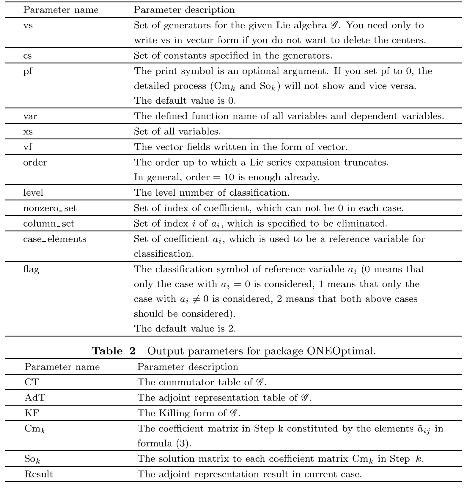
Table 1 Input parameters for package ONEOptimal.
Some main package commands and corresponding inputs are given in the following listing.In ONEOptimal,the main routine is Get Optimal(vs,cs,pf).This procedure calls six sub-procedures:
fi nd center(vs,xs,var):Singles out the centers from vs with respect to xs and var,and deletes the centers,which have no eあect on the closure of G.
commutator table(vf,xs,var):Generates commutator table for G with the(i,j)-th entry indicating[Vi,Vj].
ad table(vf,order):Computes the adjoint representation table of G with the(i,j)-th entry indicating Adexp(∈Vi)(Vj).For simplicity,the truncated power series expansions up to order in the calculation result are all replaced by the original series name.
K form(X):Computes the Killing form on the basis of the commutator table X.
Classify(kf,C):Classif i es the original system to several cases according to Killing form kf and executes opti-mization.
show optimal():Prints out the optimized results.Other package commands and corresponding inputs are given in the following listing:
LinearCo(expr,vf,var):Writes the expression expr as a linear combination of the generators in vf with respect to var.
lie bracket cal(a,b,var):Computes the commutator of a pair of vectors a and b.Here,both a and b are single generators,while the result is returned as a linear combination expression.
Lie bracket(a,b):Computes the commutator of a and b.Here,a and b can be linear combination of generators.
ad operator(a,b,order):Acts by adjoint maps generated by a and b up to order order.Here both a and b are single generators.
ad(a,b):Acts by adjoint maps generated respectively by a and b.Here a and b can be linear combination of generators.Command ad(Vm,Eqn)can also be used to observe and adjust the coeきcient in Eqn.
replace(result,j,ex,order):Replaces the truncated series expansion trse in the coeきcient of Vjin result with the name of the original series.Here,ex represents the coeきcient of∈determined from current trse.
coeきcient obtain(eq): Computes the coeきcient matrix Cmkobtained by adjoint maps generated respectively by all generators Viand eq.
coeきcient solve(C):Solves out ε from every element(expression about∈)in the coeきcient matrix C,and provides the solution matrix to C.
deno reduce(d,C):Eliminates some Viaccording to the specif i ed generator d from the equation corresponding to matrix C.Here,for d is nonzero,it is possible to eliminate Viif d appears in the denominator of column i in solution matrix corresponding to C.
reduce(column set,C):Eliminates a best Viin column set from Eqkcorresponding to C in current step k.
reduce all(column set,C):Eliminates all Viin column set from Eqkcorresponding to C in current step k.
case classify(case elements,C,level,nonzero set,f l ag):Classif i es current case to n subcases for each reference variable aiin coeきcient set case elements:ai=0(when f l ag=0,2)and ai/=0(when f l ag=1,2).
check column(s,level,nonzero set):Checks Soswhether the current case can be simplif i ed further,that is to say,whether there are some columns that can be eliminated.Here,s represents the step number.
check row(s):Picks out the best row number whose corresponding adjoint representation has most ε in Cms.
optimal calculate(s,nonzero set):Calculates the reduced adjoint representation result according to nonzero set for the case in Step s.
5 Illustrative Examples
In this section,several diあerent kinds of examples are given to illustrate the eあectiveness of our package ONEOptimal.
5.1 Examples with One Variable in Killing Form
Example 1 Consider the four-dimensional symmetry algebra g of the Korteweg-de Vries equation

which is generated by the vector f i elds

From Table 3

Table 3 The commutator table for Example 1.
the Killing form is obtained

An optimal system of one-dimensional subalgebras of this algebra is those spanned by:

Depending on the sign of a3,we can make the coeき-cient of V3either+1,?1 or 0.Thus the result is consistent with the result given by Olver[3]

The average running time for this example is 0.2622 seconds.
Example 2 Consider the four-dimensional symmetry algebra g of the Navier–Stokes equation

which is generated by the vector f i elds

From Table 4
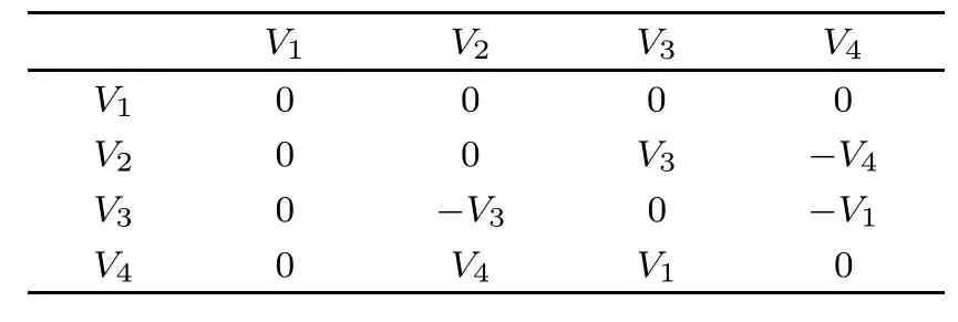
Table 4 The commutator table for Example 2.
the Killing form is obtained

An optimal system of one-dimensional subalgebras is provided by those generated by:

Depending on the sign of a4,we can make the coeき-cient of V4either+1,?1 or 0.Thus the result is consistent with the result given by Hu[22]

where α is an arbitrary constant.
The average running time for this example is 0.2356 seconds.
5.2 Examples with Two Variables in Killing Form
Example 3 Consider the seven-dimensional symmetry algebra g of the Zakharove–Kuznetsov equation[23]

which is generated by the vector f i elds
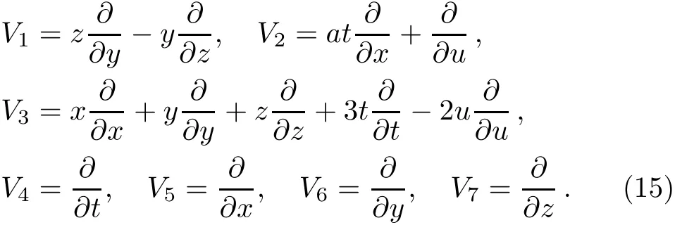
From Table 5
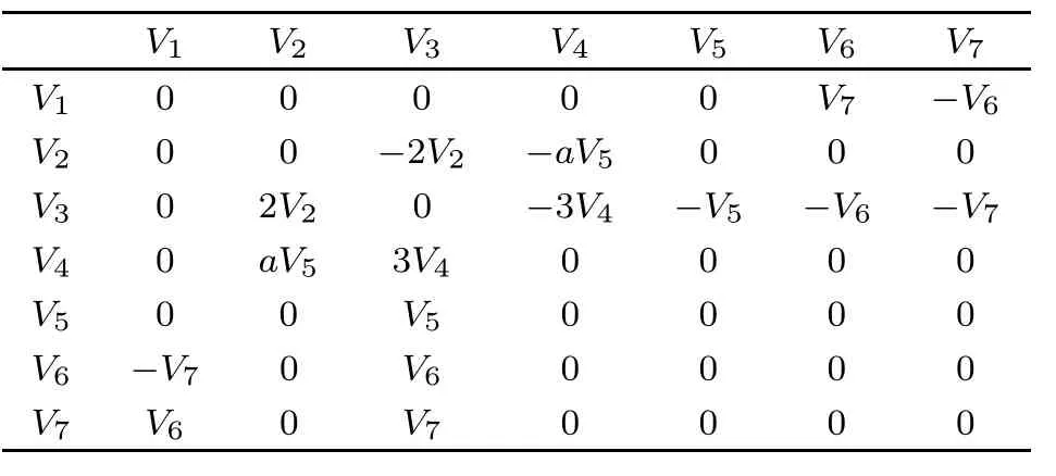
Table 5 The commutator table for Example 3.
the Killing form is obtained

An optimal system of one-dimensional subalgebras is provided by those generated by:
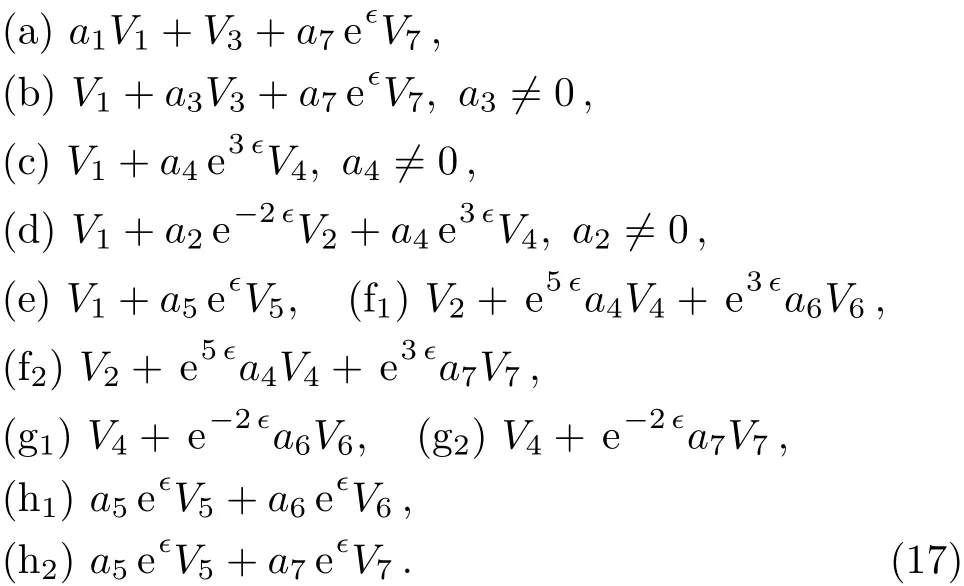
Depending on the sign of a4,a5,a6,a7,we can adjust the coeきcient of V4,V5,V6,V7to suitable value.Thus this result is consistent with Ref.[24].
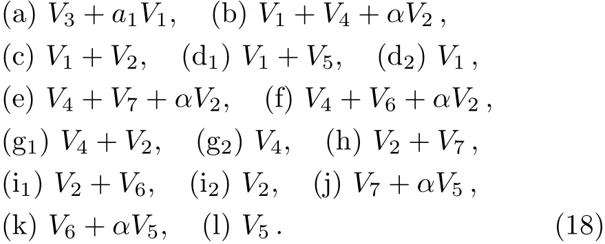
where α is an arbitrary constant.
The average running time for this example is 1.2043 seconds.
Example 4 Consider the seven-dimensional symmetry algebra g of the two layers of atmosphere model equation

which is generated by the vector f i elds

From Table 6
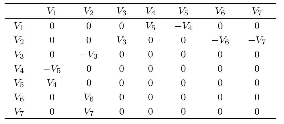
Table 6 The commutator table for Example 4.
the Killing form is obtained

A one-dimensional optimal system is those spanned by:

This is consistent with Ref.[25]after adjusting the coeきcients which contain ∈.


where λ /=0,α,β,μ are arbitrary constants.
The average running time for this example is 0.7489 seconds.
5.3 Examples with Three Variables in Killing Form
Example 5 Consider the six-dimensional algebra g of the heat equation

which is generated by the vector f i elds

From Table 7
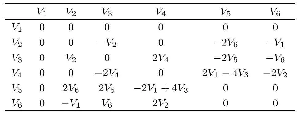
Table 7 The commutator table for Example 5.
the Killing form is obtained

A one-dimensional optimal system is:

This result is consistent with Refs.[3,11]after adjusting the coeきcients which contain ∈.

where a,b are arbitrary constants.
The average running time for this example is 0.7427 seconds.
Example 6 Consider six-dimensional algebra g of the quasilinear equation[26]

which is generated by the vector f i elds


From Table 8

Table 8 The commutator table for Example 6.
the Killing form is obtained

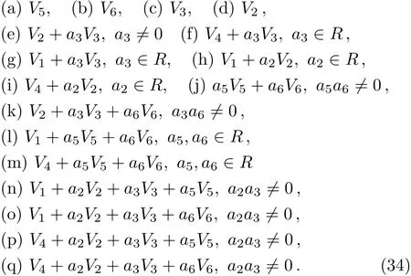
A one-dimensional optimal system is provided by:

This result is in accordance with Ref.[27]after adjusting the coeきcients which contain ∈.
The average running time for this example is 1.1356 seconds.
5.4 More Examples of Real Two-,Three-and Four-Dimensional Lie Algebras
Consider some nontrivial real Lie algebras listed in the fi rst column of Table 9,which have appeared in Ref.[28].Based on the existing nonzero commutation relations presented in the second column,the Killing forms,classi fication results from our program and running times are listed in the last three columns,respectively.Depending on the sign of a1,a2,a3,a4,we can adjust the coeきcients of V1,V2,V3,V4,which contain∈to suitable value such as?1,1,0.In comparison,the output from our program is consistent with Ref.[28].

Table 9 One-dimensional optimal systems of real two-,three-,and four-dimensional Lie algebras.Parameter description:a1,a2,a3,a4are arbitrary constants.
5.5 Examples of Some Classical Lie Algebras
Finally,we also consider some classical Lie algebras using our program.Their corresponding nonzero commutation relations,Killing forms,classif i cation results,and running times are given in Table 10.

Table 10 One-dimensional optimal systems of classical Lie algebras.
6 Conclusions
In this paper,we have presented and clarif i ed the Maple package ONEOptimal to construct one-dimensional optimal system of Lie algebra based on Olver’s method.The program ONEOptimal can compute the commutator table,adjoint representation table and Killing form automatically,while it can also execute the optimization process step by step.ONEOptimal is very easy to perform as it requires minimal user input and the output with instructions is easy to understand.The program will play a signif i cant role in the search of group invariant solutions.How to involve the cases with more variables in the Killing form and realize the mechanization of highdimensional optimal system of subalgebras is worthy of our further study.
Appendix:The Detailed Usage of Package ONEOptimal
The package ONEOptimal will work on Maple 13 or higher version.In the following two classical examples(Examples 1 and 5 in Sec.5)are given to illustrate how to use this package.The detailed input and output are demonstrated as follows.
Example 1 Consider the KdV equation(4),one can proceed as follows:
#Import the package ONEOptimal
>with(ONEOptimal):
#Defination of the function with variables
>alias(phi=phi(x,t,u));
#Defination of the vector fields
>kdv:={diff(phi,x),diff(phi,t),t*diff(phi,x)+diff(phi,u),
x*diff(phi,x)+3*t*diff(phi,t)-2*u*diff(phi,u)};
#Run the main routine Get_Optimal
>Get_Optimal(kdv,{},0); #{}--There is no constant in this algebra.
0--Do not show the detailed matrices Cm and So.
The output is:
There is no center.
The commutator table for this algebra is:
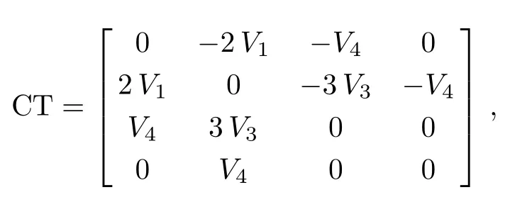
with the generators:

The adjoint representation table is constructed

The Killing form is:

Step 1

The coeきcient matrix is:

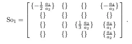
The corresponding solution matrix is:
Case 1

Case 2

Case 2.1

Case 2.2

Case 2.2.1

Case 2.2.2

In this example,depending on the sign of a3,we can make the coeきcient of V3either+1,?1 or 0 in Case 2.1.Summarize the above cases,the one-dimensional optimal system equals to:V2,V1+V3,V1?V3,V1,V3,V4.
Example 5 Consider the heat equation(25),one can proceed as follows:
#Import the package ONEOptimal
>with(ONEOptimal):
#Defination of the function with variables
>alias(phi=phi(x,t,u));
#Defination of the vector fields
>heat:={u*diff(phi,u),2*t*diff(phi,x)-x*u*diff(phi,u),x*diff(phi,x)+2*t*diff(phi,t),4*t*x*diff(phi,x)+4*t^2*diff(phi,t)-(x^2+2*t)*u*diff(phi,u),diff(phi,t),diff(phi,x)};
#Run the main routine Get_Optimal
>Get_Optimal(heat,{},0);#{}--There is no constant in this algebra.0--Do not show the detailed matrices Cm and So.
The output is:
The center of the algebra is:
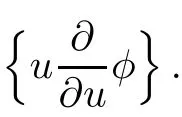
The centers can not be deleted.
The commutator table for this algebra is:

with the generators:

The adjoint representation table is constructed:

The Killing form is:

Step 1

The coeきcient matrix is:

The corresponding solution matrix is:

Case 1

Case 2

Case 2.1

Case 3

Case 3.1

Case 3.1.1

Case 3.1.2


Case 4

Case 4.1

Case 4.2

Case 4.2.1

Case 4.2.2

In this example,depending on the sign of a5,we can make the coeきcient of V5only+1 in Case 1 and either+1 or?1 in Case 3.1.1.The coeきcient of V1can be set either+1,?1 or 0 in Case 3.1.2,but arbitrary in both Case 1 and Case 2.1.Summarize the above cases,this one-dimensional optimal system equals to:V4+V5+bV1,V3+aV1,V2+V5,V2?V5,V5+V1,V5?V1,V5,V2,V6,V1,where a,b∈R.
[1]S.Lie,Arch.Math.6(1881)328.
[2]L.V.Ovsiannikov,Group analysis of diあerential equations,Academic,New York(1982).
[3]P.J.Olver,Applications of Lie Groups to Diあerential Equations,2nd ed.,Springer,New York(1993).
[4]F.Galas and E.W.Richter,Physica D 50(1991)297.
[5]J.C.Fuchs,J.Math.Phys.32(1991)1703.
[6]S.V.Coggeshall and J.Meyer-Ter-Vehn,J.Math.Phys.33(1992)3585.
[7]L.Gagnon and P.Winternitz,J.Phys.A 21(1988)1493.
[8]L.Gagnon and P.Winternitz,J.Phys.A 22(1989)469.
[9]L.Gagnon,B.Grammaticos,A.Ramani,and P.Winternitz,J.Phys.A 22(1989)499.
[10]N.H.Ibragimov,CRC Handbook of Lie Group Analysis of Diあerential Equations,CRC Press,Boca Raton(1994).
[11]K.S.Chou,G.X.Li,and C.Z.Qu,J.Math.Anal.Appl.261(2001)741.
[12]X.R.Hu and Y.Chen,Commun.Theor.Phys.52(2009)997.
[13]Z.Z.Dong and Y.Chen,Commun.Theor.Phys.54(2010)389.
[14]X.R.Hu,Y.Chen,and L.J.Qian,Commun.Theor.Phys.55(2011)737.
[15]F.Schwarz,SIAM Rev.30(1988)450.
[16]A.K.Head,Program LIE for Lie Analysis of Diあerential Equations on IBM Type PCs,User’s Manual(2000).
[17]A.K.Head,Program BIGLIE for Lie Analysis of Diあerential Equations on IBM Type PCs,User’s Manual(2000).
[18]G.Baumann,Symmetry Analysis of Diあerential Equations with Mathematica,Springer,New York(2000).
[19]E.S.Cheb-Terrab and K.von Bulow,Comp.Phys.Commun.90(1995)116.
[20]K.T.Vu,J.Butcher,and J.Carminati,Comp.Phys.Commun.176(2007)682.
[21]J.Carminati and K.Vu,J.Symbolic Comput.29(2000)95.
[22]X.R.Hu,Z.Z.Dong,and Y.Chen,Z.Naturforsch.65a(2010)1.
[23]G.C.Das,J.Sarma,Y.T.Gao,and C.Uberoi,Phys.Plasmas.7(2000)2374.
[24]Z.Z.Dong,Y.Chen,and Y.H.Lang,Chin.Phys.B 19(2010)090205.
[25]Z.Z.Dong,F.Huang,and Y.Chen,Z.Naturforsch.66a(2011)75.
[26]G.Aronsson,Ark.Mat.6(1967)551.
[27]I.L.Freire and A.C.Faleiros,Nonlinear Anal.74(2011)3478.
[28]J.Patera and P.Winternitz,J.Math.Phys.18(1977)1449.
 Communications in Theoretical Physics2014年2期
- Communications in Theoretical Physics的其它文章
- Solutions of the Schr¨odinger Equation with Quantum Mechanical Gravitational Potential Plus Harmonic Oscillator Potential
- Exact Polynomial Solutions of Schr¨odinger Equation with Various Hyperbolic Potentials?
- Dynamics of Light in Teleparallel Bianchi-Type I Universe
- Entangled Three Qutrit Coherent States and Localizable Entanglement
- Robust Quantum Computing in Decoherence-Free Subspaces with Double-Dot Spin Qubits?
- Eきcient Numerical Algorithm on Irreducible Multiparty Correlations?
