Jacques GOLDER, Maminirina JOELSON*, Marie-Christine NEEL, Liliana DI PIETRO

1. Department of Physics, University of Avignon, Avignon 84000, France

2. Mediterranean Environment and Agro-Hydro System Modelisation Laboratory, French National Institute for Agricultural Research, Avignon 84914, France

A time fractional model to represent rainfall process

Jacques GOLDER1,2, Maminirina JOELSON*1,2, Marie-Christine NEEL1,2, Liliana DI PIETRO2

1. Department of Physics, University of Avignon, Avignon 84000, France

2. Mediterranean Environment and Agro-Hydro System Modelisation Laboratory, French National Institute for Agricultural Research, Avignon 84914, France

This paper deals with a stochastic representation of the rainfall process. The analysis of a rainfall time series shows that cumulative representation of a rainfall time series can be modeled as a non-Gaussian random walk with a log-normal jump distribution and a time-waiting distribution following a tempered α-stable probability law. Based on the random walk model, a fractional Fokker-Planck equation (FFPE) with tempered α-stable waiting times was obtained. Through the comparison of observed data and simulated results from the random walk model and FFPE model with tempered α-stable waiting times, it can be concluded that the behavior of the rainfall process is globally reproduced, and the FFPE model with tempered α-stable waiting times is more efficient in reproducing the observed behavior.

rainfall process; heavy-tailed probability distribution; tempered α-stable probability law; log-normal law; Hurst exponent; continuous time random walk model; fractional Fokker-Planck equation

1 Introduction

The rainfall process is known to have a fundamental importance in natural environment. For example, it provides groundwater by causing rainwater to seep into ground in a process called infiltration, resulting in the regeneration of fresh water. Thus, rainfall structure and its mechanisms have been a subject of intense study in the past. In particular, the temporal structure of rainfall at a point has been widely investigated using models based on downscaling methods. The majority of the existing models use fractal cascade processes introduced in the 1970s by Kahane (1974), Peyriere (1974), and Mandelbrot (1974). The fractal cascade model and its generalization to a multifractal model (Schertzer and Lovejoy 1987) have been widely used to reproduce the variability of different rainfall phenomena (Gupta and Waymire 1993; Perica and Foufoula-Georgiou 1996; Gaume et al. 2007). The success of the cascade model is largely related to the multifractal theory and its simple implementation that requires only few parameters. The multifractal theory implies power law scaling in rainfall statistics. However, deviations from power law scaling in statistical moments of rainfallprocesses have been reported in recent studies (Olsson 1995; de Lima and Grasman 1999; Olsson and Burlando 2002; Marani 2005). Also, calibration and validation of cascade models are not always easy (Gaume et al. 2007).

On the other hand, diffusion models have been used to model the rainfall process. Diffusion modeling under Markovian assumptions, including the geometrical Brownian motion process, was carried out by Veneziano et al. (1996). Recently, a fractional diffusion model was also used successfully by Kundu and Bell (2006) and Kundu and Travis (2013). In this study, we focus on the representation of the rainfall process with a fractional time stochastic process with a long memory effect. First, a daily rainfall time series recorded over 40 years was analyzed. The results suggest that the data exhibit a memory effect and the behavior of the cumulative curve of rainfall displays constant characteristic periods. These immobile periods are found to follow Lévy statistics, while rainfall intensity variations follow a log-normal probability law. Such behavior is commonly observed in physical systems exhibiting subdiffusion. In particular, the constant periods in the cumulative rainfall curve indicate trapping events in which the subdiffusive test particule gets immobilized in a trap. This suggests that the temporal structure of the rainfall may be modeled by subordinated geometrical Brownian motion (Magdziarz 2009). According to this idea, in the second step of this study, the random walk model with a heavy-tailed waiting time (Metzler et al. 1999) was adopted, and a fractional Fokker-Planck equation (FFPE) (Metzler and Klafter 2000) with tempered α-stable waiting times was derived from it. Finally, the simulated results from the random walk model and FFPE model with tempered α-stable waiting times were compared with the observed data.

2 Time series analysis

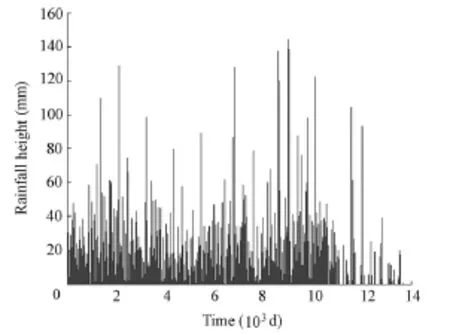
Fig. 1 Rainfall height time series

This study started with the analysis of rainfall data recorded over 40 years (1968 to 2008) in Avignon, in the southeast of France (43°54′58″N, 4°52′58″E). The rainfall time series variation is given in Fig. 1. To analyze the rainfall time series, we first decomposed it into sequences of intensity and occurrence. We defined the occurrence as the random time intervalbetween two rainfall events. Then, two analysis methods were applied to the sequences of intensity and occurrence. The first analysis method deals with the probabilistic structure of the rainfall intensity and rainfall occurrence sequences. The second one is intended to estimate the effect of long-range dependence in the data. These analyses aim to highlight statistical properties of rainfall dynamics. Results of analysis provide a basis for the mathematical model.

2.1 Probability density function

In order to characterize the probabilistic structure of the rainfall process, we estimated the histograms of the intensity and occurrence series. It was found that these histograms show positively skewed distributions. In addition, the histogram of the rainfall time series shows heavy-tailed distribution. This is also the case for the occurrence series, but not for the intensity sequences. Such results are in agreement with those obtained in the French Mediterranean area by Delrieu et al. (2005).

The probability distribution of a random variable X is said to be a heavy-tailed one if its density function possesses asymptotic behaviour following a power law as written in Eq. (1).

where P(X ＞ x) is the probability that random variable X has a value greater than x, and λ is the exponent of the power-law function. Many probability distributions have heavy tails. Not all the statistical moments are finite in a major portion of these probability distributions; this is the case of the family of α-stable laws. Some examples of heavy-tailed distributions with finite statistical moments have log-gamma distribution, Pareto distribution, and T-distribution. The heavy-tailed property is also linked to the self-similarity property and has a long memory effect. According to our analysis results and those of earlier studies, we adopted a log-normal model (Cho et al. 2004) to fit the intensity sequences. The probability density function of the log-normal distribution is

where μ and σ are, respectively, the mean and the standard deviation of the probability distribution. An α-stable distribution was used to fit the occurrence histogram. The most common way to formulate an α-stable distribution is given by the expression of its characteristic function (Joelson and Néel 2008)

where

with α, β, ν, and γ being, respectively, the stability index (0 2α＜ ≤ ), the skewnessparameter (?1 ≤ β≤ 1), the location parameter, and the scale index. It is noted that when the stability index reaches its maximum value (α = 2), we have the Gaussian probability distribution that is a symmetrical law (β = 0). In this particular case, the last two parameters ν and γ are the mean and the standard deviation of the Gaussian probability distribution.

From rainfall waiting time series, the four parameters of the α-stable distribution are obtained using the procedures formulated in Koutrouvelis (1980), Koutrouvelis (1981), and McCulloch (1986). They are α= 0.95, β= 1, γ= 0.3627, and ν=? 5.6324. The two parameters of the log-normal distribution of the rainfall intensity variation are obtained using data fitting, and they are μ= 1.4, and σ2= 1.32.

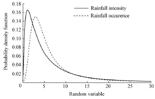
We find in particular that the skewness parameter is at its maximum value β= 1. This ensures that the positivity of the probability distribution is in agreement with the physical meaning of the rainfall occurrence as a waiting time. Probability density functions of rainfall intensity and rainfall occurrence are given in Fig. 2.

Fig. 2 Probability density functions of rainfall intensity and rainfall occurrence

2.2 Long memory effect

The long-term memory effect is quantified using the Hurst exponent (H). The Hurst exponent is referred to as an index of long-range dependence. It is defined in terms of the asymptotic behaviour of the rescaled range (Hurst 1951) as a function of the time span of a time series as follows:

where R(n) is the range of cumulative departures from the sample mean value,S(n) is the standard deviation, C is a positive constant, n is the length of the data, and E(x) indicates the expected value. According to Eq. (4), the values of the Hurst exponent range between 0 and 1.

A Hurst exponent value H close to 0.5 indicates a pure random walk (also named a Brownian time series). In such a random walk, there is no correlation between any current element and a future element. Also, there is a 50% probability that future return values will goeither up or down. Series of this type are known to be hard to predict. A Hurst exponent value H between 0 and 0.5 exists for the time series with anti-persistent behavior. This means that an increase will tend to be followed by a decrease (or a decrease will be followed by an increase). This behavior is sometimes called mean reversion, which means that future values will have a tendency to return to a longer-term mean value. The strength of this mean reversion increases as H approaches 0. A Hurst exponent value H between 0.5 and 1 indicates persistent behavior. If there is an increase from time step i-1 to i, there will probably be an increase from i to i+1. The same is true of decreases, where a decrease will tend to follow a decrease. The trend is more enhanced with the increase of the Hurst exponent value. Such a trend is known to be an indicator of long memory dependence in the time series dynamics. Series of this type are easier to predict than series falling in the other two categories. However, other phenomena such as a nonstationarity in the mean can cause behavior leading to 0.5H≠ (Klemes 1974). In order to avoid an artifact, we analyzed not only the rainfall but also the rainfall intensity variation and the time series of the rainfall occurrence. The obtained Hurst exponent values for rainfall, rainfall intensity, and rainfall occurrence are 0.545 6, 0.625 4, and 0.67, respectively, which shows that all three series exhibit persistent behaviour. These values also suggest the existence of long-range memory in the rainfall dynamics.

3 Random walk and FFPE models

According to the results of the data analysis, the cumulative precipitation curve is considered a random walk realization. To model the rainfall process, we consider a one-dimensional random process, combining advection and dispersion, which is given by the following random walk (starting from0x at time t = 0):

where Xkis the position of the walk particle at time Tk, Ikis the random jump at the kth step, Wkis the random waiting time at the kth step, τ and l are time and space steps of the random walk, and V is an average flow field with V = μτ. The particle displacement is due to the average flow field V and dispersion. A particle starting at the time instant t = 0 at the space point x0= 0 makes jumps of random size lIkat random instant Tkand is convected with the mean flow. According to the results of time series analysis, we assume the variables Wkand Ikto be independent and identically distributioned (i.i.d.) random variables following an α-stable distribution and a centered log-normal distribution with μ= 0, respectively.

Thereafter, we focus on the limit of the random walk when the time and space steps (τ, l )→ 0 with a constant ratio of l2τ= D. In this case, an FFPE model can be derived by estimating the particle flux:

where0is the Riemann-Liouville fractional derivative for a given function ()gt, and ( ),xtφ is the probability density function of a subordinated geometric Brownian motion. The result in Eq. (6) was also obtained by Magdziarz (2009) starting from a Black-Scholes model subordinated by a heavy-tailed waiting time process.

4 FFPE model with tempered α-stable waiting times

The first application of the FFPE model, as presented above, shows that the use of the α-stable law as the probability distribution of waiting time does not provide much satisfaction. Indeed, the subdiffusive model with α-stable waiting times produces a result that overestimates the range of abnormality of observed data. Such a situation was observed in some attempts to represent the physical system with a subdiffusive model (Cadavid et al. 1999). Better results were obtained when using tempered α-stable waiting times instead of the initial α-stable waiting times. A tempered α-stable random variable is conveniently defined via the Laplace transform (h) of its probability density function as follows:

where u represents the Laplace variable, and δ( 0δ＞ ) is the tempering parameter. Statistical moments of all orders of a tempered α-stable random variable are finite. Also, it is noted that according to Gajda and Magdziarz (2010), the use of the tempered α-stable waiting times allows one to derive the same form of the FFPE model given in Eq. (6), but corresponding to a tempered subdiffusion.

5 Application to data

Two types of simulations were conducted to model the cumulative precipitation. The first type was based on the random walk model of Eq. (5) using a Monte-Carlo technique. By generating realizations of random variableskW andkI, trajectories of the random walk were built, and the mean of the simulated trajectories was estimated.

FFPE simulations were also carried out. Recently, Gajda and Magdziarz (2010) have shown the equivalence between the solution to the FFPE model with tempered α-stable waiting times and the probability distribution of the subordinated Langevin process with the form Y = Z(St), where Z is the solution to the following Ito stochastic differential equation

whereB(τ) is the standard Brownian motion, and Stis the inverse of a tempered α-stable subordinator, defined asbeing a strictly increasing tempered α-stable process. We used this result to simulate trajectories of particles following the FFPE probability density function. Realizations of the stochastic process Y are simulated using the procedure described by Magdziarz et al. (2007).

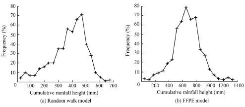
Results obtained from the random walk model of Eq. (5) and the FFPE model of Eq. (8) at t = 300 d are shown in Fig. 3. It can be seen from Fig. 3 that the FFPE model appears more capable of taking into account extrem events. For the random walk model, values of parameters are given in Section 2.1. For the FFPE model, values of the tempering parameter δ and the coefficient D providing the best fit of the data were found to be δ= 10?5and D = 0.095. In both simulations, 400 trajectories was used to estimate the mean trajectory. Each trajectory was made of more than 17 000 points, allowing us to simulate 50 years of daily precipitation time series.

Fig. 3 Cumulative rainfall height simulated with random walk and FFPE models at t = 300 d

From Fig. 4, the results of simulations show that the behavior of the rainfall process is globally reproduced. The FFPE model is found to be more efficient in reproducing the observed behavior. However, the declining trend of observed data from years 1997 to 2008 is not well simulated by the two models. This discrepancy is not easy to explain. Despite this fact, our models are a generalization of the geometrical Brownian model used by Veneziano et al. (1996) and differ sensibly from the usual multiplicative cascade models that do not take account of the memory effect (Paschalis et al. 2012).

Fig. 4 Observed cumulative precipitation and those simulated with random walk and FFPE models

6 Conclusions

In this study, we decomposed a rainfall time series as sequences of intensity and occurrence. The basic idea of the study was to consider these sequences as a realization of a random walk, in which rainfall intensity values are the random jumps. The random duration between two rainfall events that we call occurrences is the waiting time. Starting from this viewpoint, we analyzed the probability distribution of the intensity and occurrence sequences. A log-normal probability distribution was found to govern the variation of the rainfall intensity while occurrences were found to follow an α-stable probability distribution. We also estimated the existence of a long-range dependence in the time series using the Hurst exponent. The results suggest that the rainfall process may be represented by an anomalous subdiffusive model. Owing to this idea, simulations with a non-Gaussian random walk model and an FFPE model with tempered α-stable waiting times were carried out to attempt to reproduce observed data. The results show that the behavior of the rainfall process is globally reproduced and the FFPE model is found to be more efficient in reproducing the observed behavior.

Cadavid, A. C., Lawrence, J. K., and Ruzmaikin, A. A. 1999. Anomalous diffusion of solar magnetic elements. The Astrophysical Journal, 521(2), 844-850. [doi:10.1086/307573]

Cho, H. K., Boxman, K. P., and North, G. R. 2004. A comparison of Gamma and lognormal distributions for characterizing satellite rain rates from the tropical rainfall measuring mission. Journal of Applied Meteorology, 43(11), 1586-1597. [doi:10.1175/JAM2165.1]

de Lima, M. I. P., and Grasman, J. 1999. Multifractal analysis of 15-minute and daily rainfall from a semi-arid region in Portugal. Journal of Hydrology, 220(1-2), 1-11.

Delrieu, G., Nicol, J., Yates, E., Kirstetter, P. E., Creutin, J. D., Anquetin, S., Obled, C., Saulnier, G. M., Ducrocq, V. Gaume, E., et al. 2005. The catastrophic flash-flood event of 8-9 September 2002 in the Gard region, France: A first case study for the Cévennes-Vivarais Mediterranean Hydrometeorological Observatory. Journal of Hydrometeorology, 6(1), 34-52. [doi:10.1175/JHM-400.1]

Gajda, J., and Magdziarz, M. 2010. Fractional Fokker-Planck equation with tempered α-stable waiting times: Langevin picture and computer simulation. Physical Review E, Statistical, Nonlinear, and Soft Matter Pgysics, 82(1 Pt 1) , 011117. [doi:10.1103/PhysRevE.82.011117]

Gaume, E., Mouhous, N., and Andrieu, H. 2007. Rainfall stochastic disaggregation models: Calibration and validation of a multiplicative cascade model. Advances in Water Resources, 30(5), 1301-1319.

Gupta, V. K., and Waymire, E. C. 1993. A statistical analysis of mesoscale rainfall as a random cascade. Journal of Applied Meteorology, 32(2), 251-267. [doi:10.1175/1520-0450(1993)032＜0251: ASAOMR＞2.0.CO;2]

Hurst, H. E. 1951. Long-term storage capacity of reservoirs. Transactions of the American Society of Civil Engineers, 116, 770-799.

Joelson, M., and Néel, M. C. 2008. On alpha stable distribution of wind driven water surface wave slope. Chaos: An Interdisciplinary Journal of Nonlinear Science, 18(3), 033117. [doi:10.1063/1.2955742].

Kahane, J. P. 1974. Sur le modèle de turbulence de Benoit Mandelbrot. Comptes Rendus hebdomadaires des Séances de l’Académies des Sciences, Série A, 278, 621-623. (in French)

Klemes, V. 1974. The Hurst phenomenon: A puzzle? Water Resources Research, 10(4), 675-688. [doi: 10.1029/WR010i004p00675]

Koutrouvelis, I. A. 1980. Regression-type estimation of the parameters of stable laws. Journal of the American Statistical Association, 75(372), 918-928.

Koutrouvelis, I. A. 1981. An iterative procedure for the estimation of the parameters of stable laws. Communication in Statistics-Simulation and Computation, 10(1), 17-28. [doi:10.1080/ 03610918108812189]

Kundu, P. K., and Bell, T. L. 2006. Space-time scaling behavior of rain statistics in a stochastic fractional diffusion model. Journal of Hydrology, 322(1-4), 49-58. [doi:10.1016/ j.jhydrol.2005.02.031]

Kundu, P. K., and Travis, J. E. 2013. A stochastic fractional dynamics model of rainfall statistics. Geophysical Research Abstracts, 15, EGU2013-1491.

Magdziarz, M., Weron, A., and Weron, K. 2007. Fractional Fokker-Planck dynamics: Stochastic representation and computer simulation. Physical Review E, 75(1), 016708. [doi:10.1103/PhysRevE.75.016708]

Magdziarz, M. 2009. Black scholes formula in subdiffusive regime. Journal of Statistical Physics, 136(3), 553-564. [doi:10.1007/s10955-009-9791-4]

McCulloch, J. H. 1986. Simple Consistent Estimators of Stable Distribution Parameters. Communications in Statistics-Simulation and Computation, 15(4), 1109-1136.

MandelBrot, B. B. 1974. Intermittent turbulence in self-similar cascades: Divergence of higher moments and dimension of the carrier. Journal of Fluid Mechanics, 62(2), 331-358.

Marani, M. 2005. Non-power-law-scale properties of rainfall in space and time. Water Resources Research, 41(8), W08413. [doi:10.1029/2004WR003822]

Metzler, R., Barkai, E., and Klafter, J. 1999. Anomalous diffusion and relaxation close to thermal equilibrium: A fractional Fokker Planck equation approach. Physical Review Letters, 82, 3563-3567. [doi:10.1103/ PhysRevLett.82.3563]

Metzler, R., and Klafter, J. 2000. The random walk’s guide to anomalous diffusion: A fractional dynamics approach. Physical Reports, 339, 1-77. [doi:10.1016/S0370-1573(00)00070-3]

Olsson, J. 1995. Limits and characteristics of the multifractal behaviour of a high-resolution rainfall time series. Nonlinear Processes in Geophysics, 2(1), 23-29. [doi:10.5194/npg-2-23-1995]

Olsson, J., and Burlando, P. 2002. Reproduction of temporal scaling by a rectangular pulses rainfall model. Hydrological Processes, 16(3), 611-630. [doi:10.1002/hyp.307]

Paschalis, A., Molnar, P., and Burlando, P. 2012. Temporal dependence structure in weights in a multiplicative cascade model for precipitation. Water Resources Research, 48(1), W01501. [doi:10.1029/ 2011WR010679]

Perica, S., and Foufoula-Georgiou, E. 1996. Model for multiscale disaggregation of spatial rainfall based on coupling meteorological and scaling descriptions. Journal of Geophysical Research: Atmospheres, 101(D21), 26347-26361. [doi:10.1029/96JD01870]

Peyriere, J. 1974. Turbulence et dimension de Hausdorff. Comptes Rendus hebdomadaires des Séances de l’Académies des Sciences, Série A, 278, 567-569. (in French)

Schertzer, D., and Lovejoy, S. 1987. Physical modeling and analysis of rain and clouds by anisotropic scaling multiplicative processes. Journal of Geophysical Research: Atmospheres, 92(D8). 9693-9714. [doi:10.1029/JD092iD08p09693]

Veneziano, D., Bras, R. L., and Niemann, J. L. 1996. Nonlinearity and self-similarity of rainfall in time and a stochastic model. Journal of Geophysical Research: Atmospheres, 101(D21), 26371-26392. [doi:10.1029/96JD01658]

(Edited by Yan LEI)

——

*Corresponding author (e-mail: maminirina.joelson@univ-avignon.fr)

Received Oct. 20, 2012; accepted Jun. 3, 2013