Salvatore Mellino, Maddalena Ripa, Sergio Ulgiati

Department of Sciences and Technologies, Parthenope University of Naples, Centro Direzionale - Isola C4 (80143), Napoli, Italy

Spatial Accounting of Environmental Pressure and Resource Consumption Using Night-light Satellite Imagery

Salvatore Mellino?, Maddalena Ripa, Sergio Ulgiati

Department of Sciences and Technologies, Parthenope University of Naples, Centro Direzionale - Isola C4 (80143), Napoli, Italy

Submission Info

Communicated by Pier Paolo Franzese

Emergy

GIS

Remote Sensing

Night-lights

LDI

Spatial Planning

Disturbance Gradient

Modern societies and economies are highly dependent on fossil energy for their survival. Unfortunately fossil energy resources and minerals are non-renewable and represent finite stocks. Consequently, societies and economies (production, trade and consumption modes) should be reorganized according to the awareness of less resource availability in the future. “Degrowth” and “prosperous way down patterns” have been suggested in order to avoid economic collapse and global societal turmoil and conflicts. This work assesses the dependence of a regional economy (Campania Region, Southern Italy) on non-renewable resources, by means of joint use of spatial modeling and Emergy Accounting. The Emergy method takes into account all the free environmental inputs (such as sunlight, wind, rain, geothermal heat) as well as the input flows of mineral and fossil energy resources, expressed in terms of their solar energy equivalents. Nonrenewable resources used within the regional economy were correlated to nighttime satellite images via GIS (Geographic Information System) methodology, to explore the load of human activities on landscape and ecological communities and to define a human disturbance gradient throughout the Region. This gradient was expressed by means of an emergy-based indicator, the Landscape Development Intensity index (LDI). Results show a high dependence of Campania Region economy from imported resources (about 85% of the total emergy used, U) and a high concentration of non-renewable flows in Napoli and Caserta Provinces. These two regional areas have much higher LDI indices, 44 and 36 respectively, suggesting the need for appropriate land use management actions capable to lower the environmental pressure to more sustainable levels.

? 2013 L&H Scientific Publishing, LLC. All rights reserved.

1 Introduction

Landscape can be considered as the basic unit for the assessment of a territorial system. Forman and Godron [1] defined landscape as a heterogeneous land area composed of a cluster of interacting ecosystems that is repeated in similar form throughout. Landscape is characterized by an area having a recurring pattern of components including both natural and human-altered land uses.

The term Region generally indicates an administrative area, which may include more than one typology of landscape. A Region may show a gradient from completely natural to highly developed areas following a spatial hierarchy in which a convergence of non-renewable energies and resources corresponds to a convergence of human economic (and disturbance) activities. The development intensity in human dominated areas determines a load on natural ecosystems altering their ecological functions [2]. The intensity of human land and resource uses can be adopted as a metric of the related disturbance gradient [3].

Odum H.T. [4,5] recognized the energy hierarchical pattern in landscape spatial organization, identifying cities as the center of such hierarchy. Agricultural areas capture the sunlight and transform this energy in more valuable biomass products, that generally converge into factories and then into consumer centers (e.g. city markets). In a like pattern, photosynthesis in forests supports the metabolic chain of herbivores, carnivores, detritivores, and ultimately the entire biodiversity. This energy transformation pattern delivers to the end of the supply chain a smaller quantity of energy (or matter) characterized by higher quality, i.e. higher control function throughout the system. Energy transformations geographically reflect the organization from small dispersed units to more centralized units, from natural and rural areas to urban centers and cities [6]. Non urbanized natural areas support and sustain the economy of urban and industrial consumption centers, as source of materials, resources and ecosystem services and as sink and buffer of impacts, emissions and wastes.

In a previous paper, we have investigated the spatial distribution of renewable flows (solar insolation, wind, geothermal heat and rainfall) developing a tool for describing the environmental worth of lands [7]. Nonetheless, our society is highly dependent on fossil energy, and it is therefore very important to include also this aspect in order to fully understand and evaluate the human pressure on natural ecosystems. The consumption of fossil resources and non-renewable materials is concentrated in different ways all over the world and shows very diverse spatial schemes also in different areas of the same nation or region, with strong links to the spatial organization of economies [5]. Before the advent of fossil energy, the geographic pattern of economic activity was driven by Earth energies: cities and societies developed closer to rivers or seacoast, in places where natural resources converged or were easily gathered (nutrients, organic matter, water) and products of economic activities were easily traded. By contrast, modern societies, with the current access to fossil resources, can develop their hierarchical centers anywhere: collection of resources and trade of products is no longer a crucial issue.

The nighttime images of the Earth from satellite photos could be used to identify the consumption centers since the light intensity might be related to the intensity of energy use [8-10] and consequently to global societal consumption [4,5]. Night-lights can be assumed as an indicator of energy consumption on the Earth surface. Several studies confirmed night-light intensity as an indicator of human and urban activities [11,12], useful to map and describe urban sprawl [13], urban dynamics [12,14-17], population density [8,18-20], economic activity [9,11,21,22] and greenhouse gas emissions [23,24], among others. This wide range of applications is due to the versatility of the night-light data source appearing as a powerful and user-friendly dataset for environmental and socio-economic studies.

In this paper, the Emergy Accounting method [4,25-27] is used to describe the state of Campania Region (Southern Italy) from a biophysical point of view, taking into account the free environmental inputs sustaining the economy (sun, rain, wind, geothermal heat, wave, among others) as well as the nonrenewable inputs of energy, minerals and goods. All the inputs driving the economy were evaluated on acommon basis and measured as solar equivalent energy. Emergy assigns value to upstream biosphere’s efforts and resource investment over time to generate natural capital and ecosystem services and thus support flows, materials, and economic services within the regional and national economic systems [27]. The non-renewable resources used within the regional economy and expressed in terms of emergy convergence per area (areal non-renewable empower density) were related to nighttime satellite images via GIS (Geographic Information System) technology to investigate the hierarchical spatial patterns of non-renewable resources consumption and to describe the human disturbance gradient throughout the regional landscapes. According to Odum [4,5] night-lights (and their concentration) are indicators of the centers of human activities in which high quality energy converges. In order to assess disturbance gradients based on non-renewable resources use, a map of the Landscape Development Intensity (LDI) index [3] was implemented for Campania Region. It provides a land use disturbance indicator, in emergy terms, identifying the areas and the extent to which human activities are concentrated [28]. On the basis of LDI maps, the conditions of landscape and ecological communities are explored and the potential impacts of human-dominated activities on ecological systems assessed.

A biosphere perspective’s accounting method is important for achieving long run sustainability and a reduction of anthropic pressure on environment and natural ecosystems. The main results obtained for Campania Region are compared in this paper to the national system’s performance, in order to understand the dynamics across scales and highlight critical points for which an appropriate environmental planning may be needed.

2 Materials and methods

Ensuing the integration between Emergy Accounting and Geographical Information Systems for spatial modeling of flows and resources [7], the methodological approach proposed hereinafter relies on satellite night-light images as a proxy for the convergence of non-renewable resources over the regional landscape.

2.1 Case study area

The Campania Region is located in the southern part of the Italian Peninsula; it has a population of 5,834,056 people and a total area of 13,595 km2[29]; the city of Naples is the regional capital. Campania is the second most populous and the most densely populated Region of Italy. Figure 1 shows the Campania Region within the Italian and European geographical context, its subdivision in provinces and its main land use categories (data from [30]). Natural areas cover the 38.15% of regional land (about 5,180 km2) and represent the less human dominated land use. There are five provinces: Napoli, Salerno, Avellino, Caserta and Benevento; the Napoli province is the most densely populated area of the Region and also the most densely populated area in Italy, with a spatial extent of 1,171 km2and a population of 3,053,247 people [29]. This means that the population density is 2,607 persons per km2and the available area for each inhabitant of the province is about 380 m2. These numbers give an idea of the urbanization and overpopulation occurred in this area, to be considered as a major cause of the loss of environmental quality of landscapes due to the high convergence of human-driven land uses.

2.2 Night-light satellite images

The sensor Operational Linescan System (OLS) belonging to the Defense Meteorological Satellite Program (DMSP) detects light emissions from the Earth surface at night. More specifically, the nighttime light (NTL) data, collected by the DMSP/OLS, measures light on Earth's surface such as those generatedby human activities, gas flares and fires. Nighttime data are made available by the National Geophysical Data Center (NGDC) of the National Oceanic and Atmospheric Administration (NOAA) (http://www.ngdc.noaa.gov). In this study the Version 4 of the NTL dataset relative to the year 2010 was used (http://ngdc.noaa.gov/eog/dmsp/downloadV4composites.html, last accessed on October, 2013). Three types of data were included in this dataset: cloud-free coverage, raw lightning data with no further filtering and stable light data. Stable light data were used since they include lights from cities, towns and other sites with persistent lighting, discarding temporary events such as fires [31,32]. The product has a spatial resolution of 30 arc-second (about 1 km), covering -180 to 180 degrees longitude and -65 to 75 degrees latitude. Each pixel value is a digital number (DN) denoting the average light intensity o##The Digital Numbers (DNs) in the night-light images are recorded over a numerical range of 0 to 63 (4 bits = 24= 64). Typically, the Digital Numbers (DNs) in a digital image are recorded over a numerical range of 0 to 255 (8 bits = 28= 256).bserved over the year ranging from 1-63 (background noise was identified and replaced with zero values). Figure 2 is an image of the used dataset relative to Italy. From this dataset, the global data were extracted according to Campania Region administrative boundaries, projected to UTM/WGS84 projection system (grid zone 33 North) and finally resampled to a pixel size of 1 km to facilitate calculation.

The low spatial resolution might be considered a shortcoming of the NTL dataset, and a higher resolution would help to perform more detailed studies over a landscape. Nevertheless, very few studies have utilized fine and medium spatial resolution nighttime light images, owing to the scarcity of available sensors [20]. Although a higher spatial resolution dataset would be a desirable step forward, the current resolution is acceptable2in view of the goal of monitoring human disturbance gradient over a wide region (larger than 13,000 km).

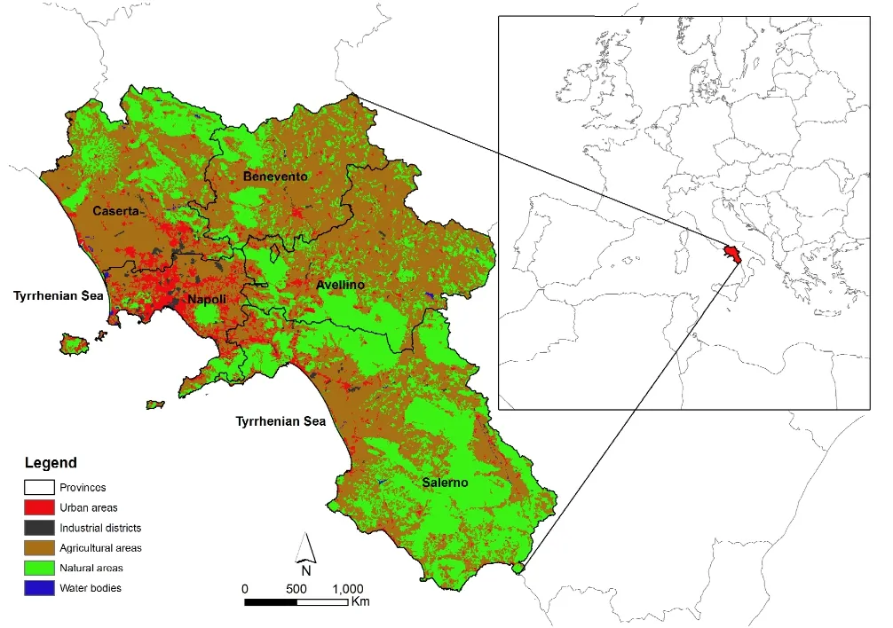
Fig. 1 Land cover map of Campania Region - data from [30].

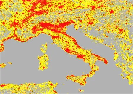
Fig. 2 DMSP-OLS nighttime imagery for Italy (stable light, 2010). Red areas correspond to high light intensity.

2.3 Emergy accounting

The emergy method [4,25,26] is a biophysical accounting approach looking at the environmental performance of a system from adonor-sideperspective, i.e. from the point of view of biosphere (the perspective of the environmental work required to support a system’s dynamics) [33]. It includes and accounts for all the resources provided directly or indirectly by nature in order to support the product or system under study, merging the past and present work of nature as well as the society’s support to its processing. By definition, emergy is the total available energy (exergy) of one kind (usually solar) previously used up directly and indirectly to make a service or product [4]. Its unit is the solar equivalent Joule (seJ). An emergy evaluation is performed by converting all the input flows of matter, available energy, labor and services into emergy units, by means of conversion factors named UEVs (Unit Emergy Values, also referred to as Emergy Intensities), and then summing up into a total emergy amount, U. UEVs quantify the amount of emergy that is required to generate one unit (J, g, $) of product or service; they are expressed as emergy per unit (seJ J-1, seJ g-1, seJ €-1). When a flow is expressed in terms of its available energy (or exergy) the UEV is also named transformity. Due to its non-conservative formalism based on amemorizationlogic [34] emergy uses algebra with specific rules when co-products of the same process reunite, in order to prevent double counting of supporting sources [35]. When two or more inflows are originated by the same emergy source (e.g. wind and rain generated by solar radiation as co-products), the risk of double-counting is avoided by adding to the total only the largest input, which by definition also includes the biosphere’s work to generate the other co-products. The total emergy investment can also be expressed per area per time (seJ area-1time-1) defining the areal empower density as a spatial measure of the resources’ concentration showing where important transformations are centered and where an environmental value should be protected [4]. In this paper, the areal empower density is quantified as seJ km-2yr-1. More specifically we can define two kinds of areal empower density, the renewable areal empower densi-ty, and the non-renewable areal empower density. The first one is a measure of renewable flows convergence throughout an area (solar radiation, rainfall, wind, geothermal heat, etc.) and it is an index of concentration of renewable resources and ecosystem services, providing useful information on the environmental worth of lands [7]. The second one is a measure of the convergence of non-renewable resources and it is an index of the anthropogenic pressure on natural ecosystems [3]. Other emergy based sustainability and performance indicators can be defined and calculated. Some of them are listed in Table 1. Further discussion on these indicators can be found in [25]

By applying GIS technologies and tools it is possible to account for the spatial dimension of the emergy method, adding valuable information that can be used for policy. The method developed in this work is capable to consider this dimension by means of satellite images, in order to explore the concentration of non-renewable flows and to assess the human pressure on natural ecosystems.

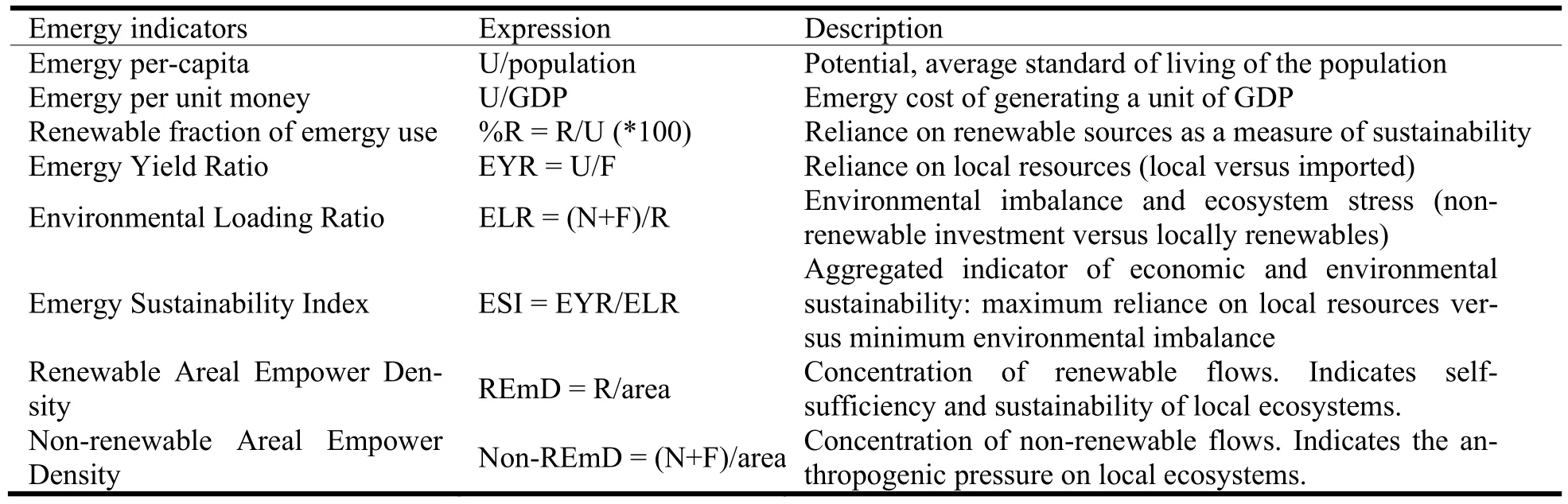
Table 1 Emergy based indicators used in this work

2.4 Assessment of human disturbance gradients

Brown and Vivas [3] developed the Landscape Development Intensity (LDI) index to quantify the disturbance gradients based on non-renewable energy and resource use in human settlements. The LDI provides an independent, quantitative, and reproducible assessment of anthropogenic influence and human disturbance gradient [36]. In this work, the nighttime light satellite imagines were used to calculate and map the LDI index, as a proxy variable for the spatial distribution of the non-renewable empower density over Campania Region. Equation 1 was implemented to spatially distribute theNonREmDvalue calculated for the whole region:

whereNonREmDi(seJ km-2yr-1) is the non-renewable areal empower density calculated for theith pixel (with a 1 km2size);NandFare, respectively, the local and the imported non-renewable emergy resource flows to the region (for Campania:N+F= 1.38E+23 seJ yr-1–Table 3),DNiis the digital number (adimensional) of the nighttime map expressing the light intensity associated to theith pixel. The denominator is the value of lighting (expressed asDN) of the entire region (for Campania, a value of 366,187 was calculated). Furthermore, Equation 2 was applied [28,37]:

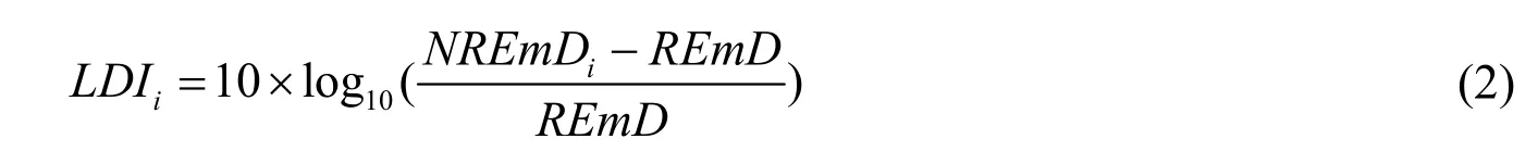
whereLDIiis the Landscape Development Intensity index for a given pixel andREmD(seJ km-2yr-1) is the renewable areal empower density of the background environment (Campania = 2.29E+17 seJ km-2yr-1– Table 3). TheLDIindex scale begins with zero and can grow without any upper limit. The zero represents areas with a value derived only from the average renewable empower of the landscape unit, in which the human presence does not alter the natural ecosystem conditions.

3 Results

3.1 Emergy results

Table 2 shows the emergy evaluation table relative to Campania Region input flows. All flows were accounted for in emergy terms and summed according to emergy algebra rules in order to avoid double counting [4], with the aim of finding out the total emergy (U) supporting the regional economy over the year 2010. The calculation procedures, the UEVs and raw data references are given in the Appendix. All UEVs in the study refer to the global emergy baseline 15.2E+24 seJ yr-1calculated as the sum, in emergy terms, of the tree main forces driving the geobiosphere: the solar insolation, the deep earth heat and the tidal energy [26].

The indicators were calculated without accounting for services. Services express the indirect labor for the manufacture and delivery of imported goods, (mainly occurring within the exporting country/region); they are converted into emergy multiplying the money paid for each input by the emergy-to-money ratio of the country/region [38]. Services are directly connected to the economy and express a society lifestyle, inflation, monetary costs, economic strategies of different countries, and are highly variable over time. Since in this work the focus is on the assessment of the human disturbance on different landscapes of the same region from a biophysical point of view, services are not included in the calculations. They can be easily added if the aim is to assess how the variability of societal welfare affects the impacts over time.

Table 2 helps identify the most important renewable, non-renewable and imported emergy flows sustaining Campania regional economy over the investigated year. It clearly appears that local (renewable and non-renewable) flows are a small, although not-negligible fraction (15%) of the total emergy (U) compared to imported emergy flows (85%). Waves represent the main renewable inflow due to the relatively long regional shoreline. According to the emergy algebra, wave emergy accounts for and includes also the other renewable flows supporting the natural dynamics of the region. Figure 3 provides a simplified interpretation of flows listed in Table 2, by grouping them into five main categories: renewable resources (items 1-7), local natural resources exploited beyond their renewal capacity (items 8-11), local non-renewable minerals and building materials (items 12-22), imported energy (items 23-29) and imported goods (items 30-39). The largest input categories are represented by the flows of imported goods (47%) and imported energy (37%).

Table 3 shows the emergy indicators calculated for Campania Region and compared to the Italian national level [38]. In order to allow a more convincing comparison, some adjustments to the Italian analysis were made: all the UEVs were updated to the 15.2E+24 seJ yr-1 baseline (Brown and Ulgiati, 2010), a more recent value for wave energy was used§, as for Campania region and indicators were recalculated without accounting for the emergy of services both for Campania and Italy.

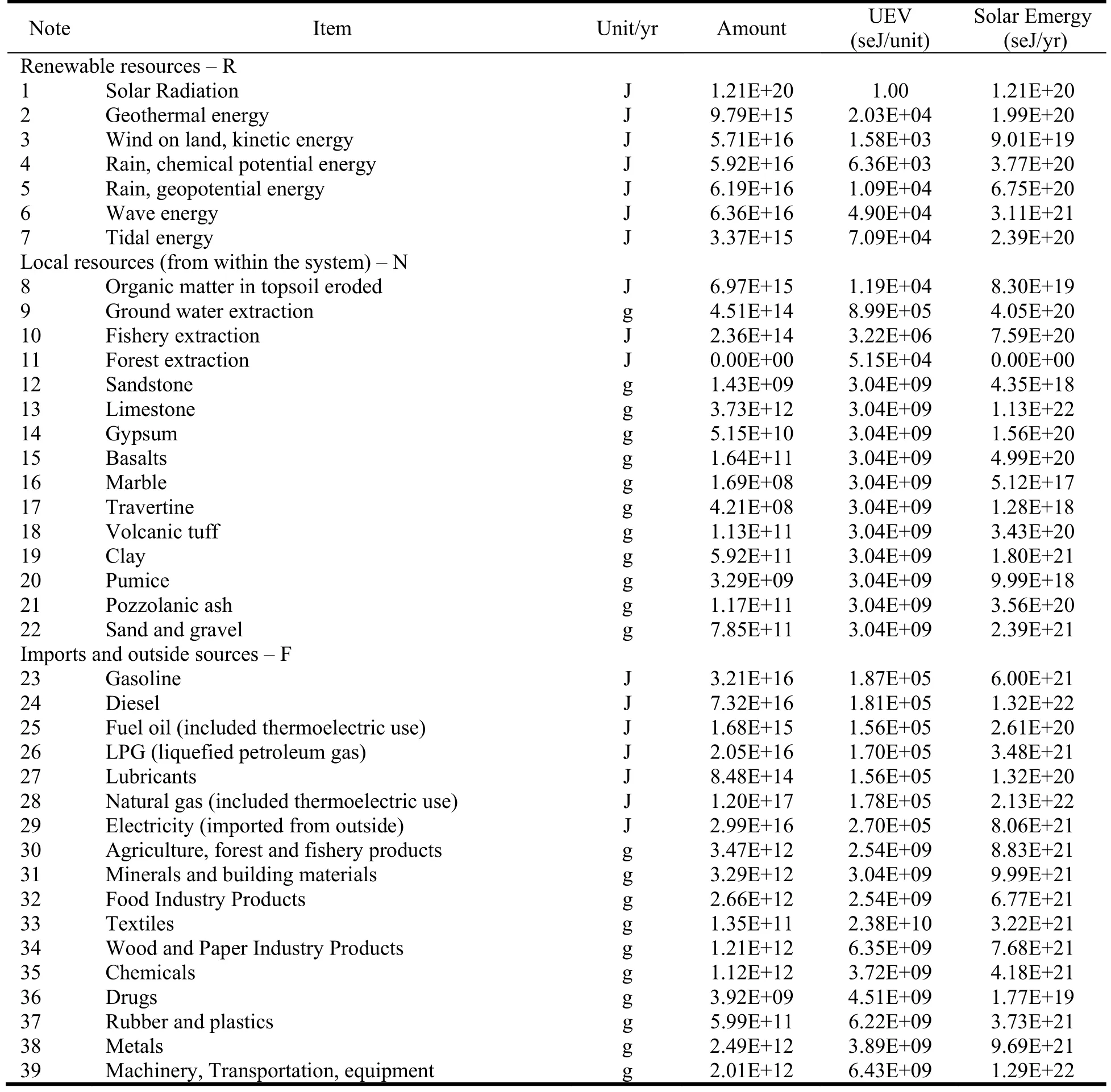
Table 2 Emergy flows supporting the economic and social system of Campania region in the year 2010. All flows are evaluated on a yearly basis. Numbers in the first column refer to calculation procedures (Appendix). UEVs values are referred to the 15.2E+24 baseline [26]

The demographic and economic indicators show a higher population density (more than 2 times) and a lowest GDP per-capita (43% less of the national average) for Campania Region compared to the national level. The emergy per-person and the emergy per-GDP are 59% and 28% lower for Campania, respectively. Conversely, the %Ren is 37% higher for Campania Region compared to the national context, while the ESI is equal for the two systems. In addition, areal indicators show a concentration of nonrenewable emergy (Non-REmD) 12% higher for Italy, while instead a 21% larger convergence of renewable emergy is observed for Campania.

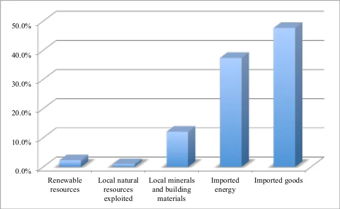
Fig. 3 Aggregated emergy signature for Campania Region.

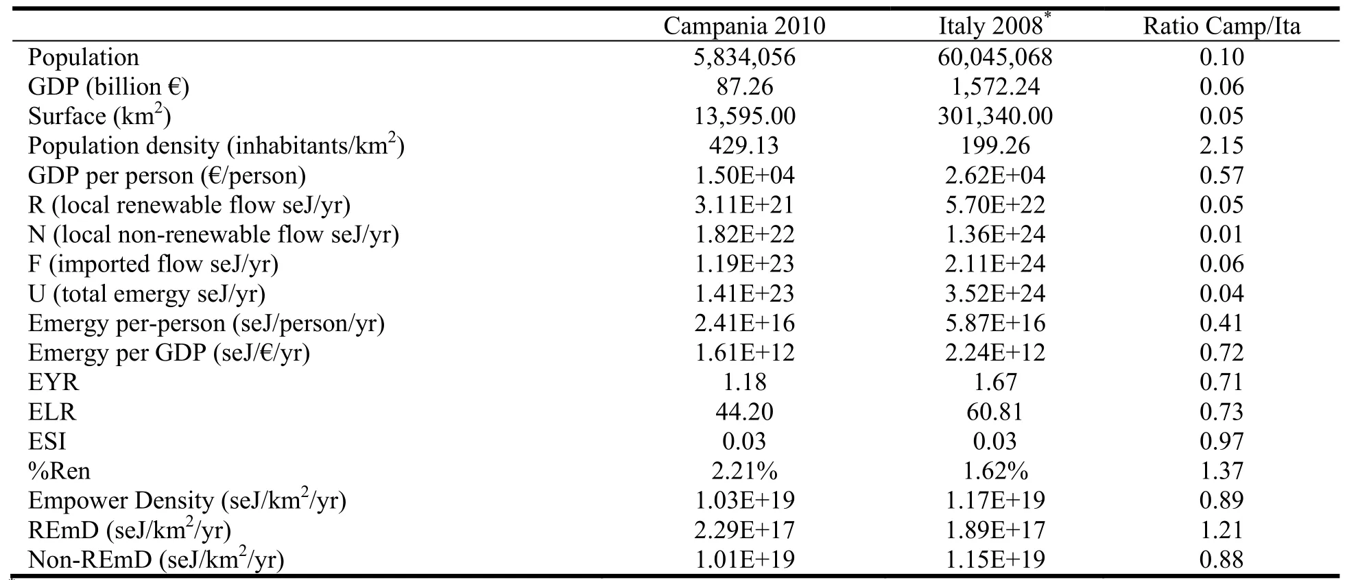
Table 3 A comparison between Campania and Italy of emergy based indicators

3.2 The human disturbance gradient map

The map of LDI Index for Campania region (Figure 4) highlights areas where the human presence and related resource consumption are highly concentrated and where natural ecosystems appear more affected by human activities and infrastructures. The LDI scale encompasses a gradient from completely natural to highly developed land use intensity, providing valuable information for landscape planning actions.

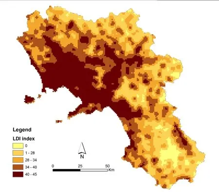
Fig. 4 LDI index map for Campania Region.

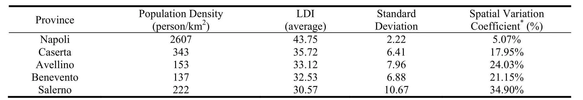
Table 4 LDI index calculated for Campania Region’s Provinces

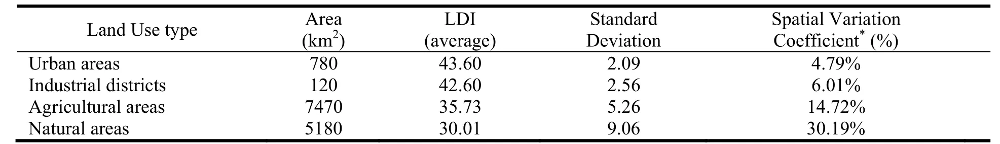
Table 5 LDI index calculated for the main land use categories of Campania Region

Table 4 shows the average values of the LDI indicator for each province of the region. Napoli Province shows the highest value (43.75) associated with the lowest standard deviation (2.22). As expressed by the spatial variation percentage, a low standard deviation value is an index of a small spatial variation and it is related to a uniform distribution of environmental conditions. On the contrary, Salerno Province shows the highest spatial variability (34.90%) associated with the lowest LDI index value (30.57). Even if the Table expresses a correlation between the high human activity concentration (with large emergy investments) and population density, this relation appears non-linear; in fact, Salerno is the third most densely populated province of the Region although it has the lowest LDI index value.

Complementary results (Table 5) were obtained by overlaying the LDI map and the main land uses of the region (Figure 1). Highest values are observable for land uses in which the human presence is dominant, confirming the capacity of the method to assess the human disturbance through landscapes.

4 Discussion

4.1 Emergy for a long-term sustainable planning

Results from Tables 2 and 3 provide information about the Campania region’s metabolism and allow to highlight material or energy flows that are critical for the regional economy under an environmental point of view. The comparison with the Italian national performance provides the possibility to analyze the regional scale taking as a reference the national average scale. The emergy indicators show a high dependence of both systems from outside and their low reliance on local resources, both renewables and nonrenewables, to drive the economy. As described in Table 1, the EYR is defined as the ratio of total emergy use to the emergy imported from outside and compares the emergy locally available with the amount that is imported. The Emergy Yield Ratio (EYR) is 1.18 for Campania, 29% lower than the national average value (1.67), underlining that the region is very inefficient in using imported resources to exploit local opportunities: every unit of natural capital and ecosystem services requires large amounts of resources from outside. From a global perspective, systems with a high dependence from outside sources, and therefore with a low value of EYR, are not competitive under a low resource availability constraint [5,41] and therefore show low sustainability in the larger resource market. The opposite situation occurs, instead, in the case of the Environmental Loading Ratio, that is lower for Campania Region than for Italy thanks to a largest share of renewable sources. According to Brown and Ulgiati [25], the ELR relates the amounts of non-renewable emergy (N+F) to the amount of renewable emergy (R). The value ELR = 0 is typical of natural ecosystems in which the renewable emergy that is locally available drives their growth with the constraints imposed by the environment. Instead, the non-renewable imported emergy drives a different development pattern, thedistanceof which from the natural ecosystem carrying capacity is quantified by the ratio (N+F)/R. From a regional economy point of view, this indicator refers to the distance of a system from an ideal system driven only by the renewable flows locally available. The higher this ratio, the bigger the distance of the societal and economic development from this ideal reference scenario. In this sense, we can say that ELR is a measure of the load on the environment and an indicator sensitive to the distance from the local carrying capacity. ELR is not, however, a direct measure of pollution in the usual chemical or biological sense. In no way ELR can specifically indicate the polluting effects of a given process since it is designed as a donor-side performance ratio: the term “stress” in Table 1 refers to the concept of excess resource convergence, which means that the local ecosystem is altered and other ecosystems are depleted. The lower value of ELR for the Campania Region compared to the national level is due to the higher availability of renewable resources per unit of area, and a consequent higher carrying capacity [42].

Additional and important information emerge from the analysis of both per-capita and per-monetaryunit emergy indicators. The emergy per-capita is an average measure of per-capita resource availability in support of potential development and standard of life. It results to be 59% lower than the Italian average showing a smaller resource availability per person within the regional context. Resource availability is a basis for agricultural production, business activities, welfare: lower availability entails less wellbeing opportunities. This indicator is, of course, affected by the population density in Campania Region. Disparities in standard of living compared to the Italian average are confirmed by the difference (-28%) of the Emergy/GDP ratio.

Figure 3 highlights the hot spots of emergy concentration: importations of energy and materials result to be critical. Table 1 shows natural gas and diesel as the main energy sources: the first one accounts for about 15% of the total emergy and it is mainly used for electricity production [43]; the latter, consumed mainly in the transport sector [44] accounts for 9% of the total U. Concerning imports, agricultural, forest and fishery products (6% of U), metals (7% of U) and machinery, transportation, equipment (9% of U) are the most relevant items. The policy-oriented information that can be derived from the emergy indicators converge towards two basic points: a) a needed reduction of fossil fuels (mainly concentrated in power plants and urban areas), and b) a reduction of imports, increased energy efficiency and increased reliance on local resources and recycling or reuse patterns. The first goal could be reached by replacing the import of fossil fuels for electricity generation, and the import of electricity itself with electricity from local renewables. The Region could take advantage from the high concentration of renewables per unit area, 21% higher than the Italian average. In the Region there are different areas where renewable flows converge, e.g. geothermal heat in Ischia and Campi Flegrei areas, wind in the eastern part of the region where the topography is mainly mountainous [7]. These areas should be suitable to increase the electricity production from renewables (wind farms, geothermal power plants, photovoltaic) and a consequent decrease of natural gas imports. This would affect the imported non-renewable emergy F and therefore improve the performance indicators of the regional system. In a like manner, the shift to mass transport systems (train, buses, urban buses and subway, possibly powered by renewable electricity) as alternative to individual transportation modalities, while requiring a non-negligible start-up investment, would significantly decrease the use of imported liquid fuels. The reduction of imports other than energy carriers requires a greater investment in local productions and increased consumers’ preferences for local products coupled to less waste of still usable resources. High population density in urban cities does not seem to be helpful to this purpose and therefore, decentralization strategies and better infrastructures (smart grids, transport, reuse/recycling networks) are urgently needed. Addressing these two aspects that jointly make up for 85% of total emergy use, may at least partially reverse the situation. Needless to say that changes in the global and local economies, although absolutely needed on the way towards sustainable development, must face the inertia ofbusiness as usualpattern and rely on a different lifestyle that does not support growth as “the first, second, and third commandment of the current economic paradigm” [41]. From a neo-classical view of the economy, the option of reduction of exports in favor of local consumption may sound impossible: in fact, the extension of the life of goods and the reduction of consumption are still against the growth-oriented principle of our economies.

4.2. The LDI index as an environmental planning indicator

The emergy method provides general indications on the interaction between economy and environment focusing on the geobiosphere’ work for resource generation. A spatial distribution of resource use evaluated in emergy terms provides valuable information about areas in which this work is concentrated and in which human activities affect natural ecosystems. The use of nighttime satellite imagery is a useful tool to assess and describe spatially the non-renewable emergy flows, increasing the capabilities of the emergy method and the possibility to develop a synthetic index of human disturbance gradient on the landscapes.

Results from the investigation of the human disturbance gradient on the Campania Region's landscapes highlight areas in which the consumption and the use of energy, raw and manufactured resources are concentrated, providing worthwhile indications for environmental landscape planning.

The LDI index is useful to identify areas exposed to environmental problems that need a careful attention in an environmental planning process. Results per province underline that the higher environmental pressures due to human presence occur in Napoli and Caserta Provinces. These two areas deal with huge environmental problems and need an appropriate land use management [45,46]. While it is evident that population density is a driver of such concentrated environmental pressure, it should not be disregarded that lifestyles, quality of resource used and low renewability of energy are “second major drivers” and require appropriate policies in order to decrease resource demand without affecting the quality of life. Identifying where and why higher LDI values occur allow to understand what and where are the most crucial processes of production and consumption develop, in so generating the unsustainable patterns revealed by LDI and other emergy indicators.

Results obtained from an overlay between the LDI map and land uses (Table 5) point out that the urban and industrial areas (including transportation infrastructures) present the higher LDI index associated with the minor standard deviation, showing a spatial uniformity of energy and resource uses for these land uses. Agricultural areas have an LDI value mainly between about 30 and 40 (considering the coefficient of spatial variability equal to 14.72% and the average value of 35.73, we can infer that the LDI values of agricultural land use are mainly between 35.73±14.72%), indicating the presence of both intensive and non-intensive agricultural systems. Finally, it is possible to point out the high standard deviation associated to natural areas (30.19%), with values for LDI falling between 30.01±30.19% (20.95 – 39.07). From one hand, this means that there are zones with a very low human activity concentration but, on the other hand, it also appears that there are some zones characterized by a high human disturbance value (about 39) for natural areas as well. These aggregate results may be profitably applied to a planning action aimed to the environmental protection and natural ecosystem preservation as well as to the most suitable exploitation of local resources and specific areas. Moreover, a quantitative measure of the intensity of human use of landscapes may be useful to map the areas in which resource use is more intensive and to monitor related trends of sustainability in consequence of ad-hoc policies aiming at saving energy and resources. Finally, considering that a low value of the LDI index is an indicator of areas with a low human pressure on ecosystems, the index can also help identify the most valuable areas for conservation purposes, in order to prevent exploitation overload.

5 Conclusion

Based on the methodologies and the approach used in this work, the following conclusions can be drawn:

a) the analysis of the metabolism of Campania Region by means of emergy accounting method has shown a high dependence of the regional economy from imported resources (85% of the total emergy U);

b) the comparison with the Italian national level has shown the lower level in standard of living of the local population;

c) regional administrators should invest efforts into a reduction of use of energy from fossil fuels and a reduction in imports, enhancing the value of local activities;

d) adding a spatial dimension to emergy method represents a powerful and important innovation for policy making;

e) the night-light satellite images are found to be a suitable proxy of concentration of non-renewable resource uses;

f) the LDI index is a valid measure to map the intensity of human use of landscapes and highlight the human disturbance gradient throughout the region, providing quantitative information for planning.

Finally, in light of results achieved, the use of night-light satellite images as a proxy variable for calculating indicators of environmental quality might be considered a powerful and very practical tool. The possibility to improve the quality of results by using images with a higher resolution should also be explored. By increasing the spatial quality of raw data it could become easier to investigate smaller fractions of a regional area like, for instance, a municipality, an agricultural district, or a specific local ecosystem.

Appendix

1. Solar radiation: Land area = 1.36E+6 ha [29]; Continental shelf area = 3.68E+05 ha at 200 m depth (our GIS elaboration); Areal available energy density of net radiation (minus albedo) = 7.01E+13 J/ha/yr [7]; Available Energy (J/yr) = Area incl. shelf (ha) * Areal available energy density (J/ha/yr) = 1.21E+20; UEV = 1.00 seJ/J by definition [4,26]

2. Geothermal energy: Land area = 1.36E+6 ha [29]; Areal available energy density of heat flow = 7.20E+09 J/ha/yr [7]; Available Energy (J/yr) = Land area (ha) * Areal available energy density (J/ha/yr) = 9.79E+15; UEV = 2.03E+04 seJ/J [26]

3. Wind on land, kinetic energy: Land area = 1.36E+6 ha [29]; Areal available energy density of wind = 7.20E+09 J/ha/yr [7]; Available Energy (J/yr) = Land area (ha) * Areal available energy density (J/ha/yr) = 9.79E+15; UEV = 1,578 seJ/J [7]

4. Rain, chemical potential energy (Calculated as available energy associated to evapotranspiration on land + available energy associated to evaporation on continental shelf): Land area = 1.36E+6 ha [29]; Continental shelf area = 3.68E+09 m2at 200 m depth (our GIS elaboration); Areal available energy density of evapotranspiration on land = 3.42E+10 J/ha/yr [7]; Rainfall on continental shelf assumed as 45% of precipitation on land = 0.70 m/yr [47]; Gibbs free energy of rainwater relative to salt water in seas receiving rain = 4,940 J/kg [4]; Available Energy on land (J/yr) = Land Area (ha) * Areal available energy density (J/ha/yr) = 4.65E+16; Available Energy on shelf (J/yr) = Shelf area (m2) * Rainfall (m/yr) * Gibbs no. (J/kg) * water density (1,000 kg/m3) = 1.27E+16; Total Available Energy (land + shelf) (J/yr) = 5.92E+16; UEV = 6,360 seJ/J [7]

5. Rain, geopotential energy: Land area = 1.36E+6 ha [29]; Areal available energy density of geopotential energy = 4.55E+10 J/ha/yr [7]; Available Energy (J/yr) = Land area (ha) * Areal available energy density (J/ha/yr) = 6.19E+16; UEV = 10,909 seJ/J [7]

6. Wave energy: Shore length 4.48E+05 m [29]; Wave power = 4.50E+03 W/m [39]; Available energy absorbed at the shore (J/yr) = Shore length (m) * Wave power (W/m) * Time in second (3.14E+07 s/yr) = 6.36E+16; UEV = 4.90E+04 seJ/J (After [48])

7. Tidal energy: Continental shelf area = 3.68E+09 m2at 200 m depth (our GIS elaboration); Average Tide Range = 0.50 m (http://www.idromare.it); Density of sea water = 1.03E+03 kg/m3; Tides per year = 730 (est. of 2 tides/day in 365 days); Available Energy (J/yr) = Continental Shelf Area (m2) * (0.5) * Tides/year * (Average Tide Range)2(m2) * Density of sea water * Gravity (9.8 m/s2) = 3.37E+15; UEV = 7.09E+04 seJ/J (After [48])

8. Organic matter in topsoil eroded: Harvested cropland = 7.47E+09 m2(estimated from [30]); Soil loss = 795 g/m2/yr (http://eusoils.jrc.ec.europa.eu/ESDB_Archive/serae/grimm/italia/erprov.htm); Total soil loss = 5.94E+12 g/yr Average organic carbon content = 3% http://eusoils.jrc.ec.europa.eu/; Organic Carbon (OC) in soil lost = 1.78E+11 g/yr; Organic Matter (OM) in soil lost = 3.08E+11 g/yr (1 OC : 1.73 OM); Energy of OM (J/yr) = OM in soil lost (g/yr) * 5.4 (Kcal/g) * 4186 (J/Kcal) = 6.97E+15; UEV = 1.19E+04 seJ/J (After [4])

9. Ground water extraction (amount of annual withdrawal exceeding annual recharge by rain): Total water withdrawn = 8.72E+08 m3/yr (http://www.istat.it/it/files/2012/03/focus_acqua_2012.pdf?title=Le+statistiche+dell’Istat+sull%27acqua+-+21%2Fmar%2F2012+-+Testo+integrale.pdf); Rainfall = 1.55 m/yr (Campania Region Civil Protection Office, 2010); Land area = 1.36E+10 m2([29]); Total rain on land = 2.11E+10 m3/yr; Groundwater recharge (2% of total precipitation) = 4.21E+08 m3/yr; Total extraction (water withdrawn - groundwater recharge) = 4.51E+08 m3/yr; Water density 1.00E+06 g/m3; Mass of water extracted = 4.51E+14 g/yr; UEV = 8.99E+05 seJ/g (After [50]).

10. Fishery extraction (It is assumed that 80% of fishery products in the Campania coastal water exceeds the annual re-production of fish. Therefore, the 80% of the total catch must be considered nonrenewable): Fishery (total catch) = 14,089 t/yr (http://agri.istat.it/jsp/dawinci.jsp?q=plP060000010000010000andan=2010andig=1andct=743andid= 13A); Fishery extraction (80% of total catch) = 11,271.2 t/yr = 1.13E+10 g/yr; Energy content of fish (average value) = 5.00 kcal/g; Fishery extraction (energy) = 2.36E+14 J/yr; UEV = 3.22E+06 seJ/J (After [49])

11. Forest extraction (Extraction means amount of annual withdrawal exceeding annual forest regrowth): Total wood withdrawal = 1.06E+07 kg/yr (http://agri.istat.it/sag_is_pdwout/jsp/NewExcel.jsp?id=7Aandanid=2010); Dry matter (30% humidity) = 7.40E+09 g/yr; Average annual biomass produced in temperate forests = 30 kg/m2; Forest area in Campania = 5.50E+07 m2(estimated from [30]); Total biomass produced in Campania forests = 1.65E+12 g/yr; Extraction = 0.0 g/yr (annual forest regrowth ＞ annual wood withdrawal); UEV = 5.15E+04 seJ/J (After [4])

12. Sandstone: Total extraction = 1.43E+03 t/yr (http://www.statistica.regione.campania.it/pubblicazioni/annuario/Annuario2007.pdf) = 1.43E+09 g/yr; UEV = 3.04E+09 seJ/g (see note at the end of the Appendix)

13. Limestone: Total extraction = 6.15E+06 t/yr (http://www.statistica.regione.campania.it/pubblicazioni/annuario/Annuario2007.pdf) = 6.15E+12 g/yr; Exported without use = 2.42E+12 g/yr (Estimated from http://www.istat.it/it/archivio/52361); Total limestone used within the Region = 3.73E+12 g/yr; UEV = 3.04E+09 seJ/g (see note at the end of the Appendix)

14. Gypsum: Total extraction = 5.15E+04 t/yr (http://www.statistica.regione.campania.it/pubblicazioni/annuario/Annuario2007.pdf) = 5.15E+10 g/yr; UEV = 3.04E+09 seJ/g (see note at the end of the Appendix)

15. Basalts: Total extraction = 1.64E+05 t/yr (http://www.statistica.regione.campania.it/pubblicazioni/annuario/Annuario2007.pdf) = 1.64E+11 g/yr; UEV = 3.04E+09 seJ/g (see note at the end of the Appendix)

16. Marble: Total extraction = 1.69E+02 t/yr (http://www.statistica.regione.campania.it/pubblicazioni/annuario/Annuario2007.pdf) = 1.69E+08 g/yr; UEV = 3.04E+09 seJ/g (see note at the end of the Appendix)

17. Travertine: Total extraction = 4.21E+02 t/yr (http://www.statistica.regione.campania.it/pubblicazioni/annuario/Annuario2007.pdf) = 4.21E+08 g/yr; UEV = 3.04E+09 seJ/g (see note at the end of the Appendix)

18. Volcanic tuff: Total extraction = 1.13E+05 t/yr (http://www.statistica.regione.campania.it/pubblicazioni/annuario/Annuario2007.pdf) = 1.13E+11 g/yr; UEV = 3.04E+09 seJ/g (see note at the end of the Appendix)

19. Clay: Total extraction = 5.92E+05 t/yr (http://www.statistica.regione.campania.it/pubblicazioni/annuario/Annuario2007.pdf) = 5.92E+11 g/yr; UEV = 3.04E+09 seJ/g (see note at the end of the Appendix)

20. Pumice: Total extraction = 3.29E+03 t/yr (http://www.statistica.regione.campania.it/pubblicazioni/annuario/Annuario2007.pdf) = 3.29E+09 g/yr; UEV = 3.04E+09 seJ/g (see note at the end of the Appendix)

21. Pozzolanic ash: Total extraction = 1.17E+05 t/yr (http://www.statistica.regione.campania.it/pubblicazioni/annuario/Annuario2007.pdf) = 1.17E+11 g/yr; UEV = 3.04E+09 seJ/g (see note at the end of the Appendix)

22. Sand and gravel: Total extraction = 7.85E+05 t/yr (http://www.statistica.regione.campania.it/pubblicazioni/annuario/Annuario2007.pdf) = 7.85E+11 g/yr; UEV = 3.04E+09 seJ/g (see note at the end of the Appendix)

23. Gasoline: Total used (mass) = 6.90E+05 t/yr (http://dgerm.sviluppoeconomico.gov.it/dgerm/bollettino/2010/trimestre4/pagina70-71.htm) = 6.90E+08 kg/yr; HHV = 46.54 MJ/kg; Total used (energy) = 3.21E+10 MJ/yr = 3.21E+16 J/yr; UEV = 1.87E+05 seJ/J [51]

24. Diesel: Total used (mass) 1.60E+06 t/yr (http://dgerm.sviluppoeconomico.gov.it/dgerm/bollettino/2010/trimestre4/pagina80-81.htm) = 1.60E+09 kg/yr; HHV = 45.77 MJ/kg; Total used (energy) = 7.32E+10 MJ/yr = 7.32E+16 J/yr; UEV = 1.81E+05 seJ/J [51]

25. Fuel oil (included thermoelectric use): Total used (mass) = 4.08E+05 t/yr (http://dgerm.sviluppoeconomico.gov.it/dgerm/bollettino/2010/trimestre4/pagina90-91.htm) = 4.08E+08 kg/yr; HHV = 45.54 MJ/kg; Total used (energy) = 2.05E+10 MJ/yr = 2.05E+16 J/yr; UEV = 1.56E+05 seJ/J [51]

26. LPG (liquefied petroleum gas): Total used (mass) = 3.68E+04 t/yr (http://dgerm.sviluppoeconomico.gov.it/dgerm/bollettino/2010/trimestre4/pagina90-91.htm) = 3.68E+07 kg/yr; HHV = 50.15 MJ/kg; Total used (energy) = 1.68E+09 MJ/yr = 1.68E+15 J/yr; UEV = 1.70E+05 seJ/J [51]

27. Lubricants: Total used (mass) = 1.84E+04 t/yr (http://dgerm.sviluppoeconomico.gov.it/dgerm/bollettino/2010/trimestre4/pagina90-91.htm) = 1.84E+07 kg/yr; HHV = 46.10 MJ/kg; Total used (energy) = 8.48E+08 MJ/yr = 8.48E+14 J/yr; UEV = 1.56E+05 seJ/J [51]

28. Natural gas (included thermoelectric use): Total used (volume) = 3.14E+09 m3/yr (http://dgerm.sviluppoeconomico.gov.it/dgerm/consumigas.asp); Density = 0.789 = kg/m3Total used (mass) = 2.48E+09 kg/yr; HHV = 48.3 MJ/kg; Total used (energy) = 1.20E+11 MJ/yr = 1.20E+17 J/yr; UEV = 1.78E+05 seJ/J [51]

29. Electricity (imported from outside): Total imported = 8.30E+03 GWh/yr (http://www.terna.it/LinkClick.aspx?fileticket=Th%2fHJtpkmo8%3dandtabid=418andmid=2501) = 2.99E+16 J/yr; UEV = 2.70E+05 seJ/J (After [52])

30. Agriculture, forest and fishery products: Total imported = 3.47E+09 kg/yr (Estimated from http://www.coeweb.istat.it and http://www.istat.it/it/archivio/52361) = 3.47E+12g/yr; UEV = 2.54E+09 seJ/g (Average UEV from [53])

31. Minerals and building materials: Total imported = 3.29E+09 kg/yr (Estimated from http://www.coeweb.istat.it and http://www.istat.it/it/archivio/52361) = 3.29E+12 g/yr; UEV = 3.04E+09 seJ/g (see note at the end of the Appendix)

32. Food Industry Products: Total imported = 2.66E+09 kg/yr (Estimated from http://www.coeweb.istat.it and http://www.istat.it/it/archivio/52361) = 2.66E+12 g/yr; UEV = 2.54E+09 seJ/g (Average UEV from [53])

33. Textiles (as cotton): Total textiles used within the Region = 1.35E+08 kg/yr (Estimated from http://www.coeweb.istat.it and http://www.istat.it/it/archivio/52361) = 1.35E+11 g/yr; Energy content of cotton = 17.00 MJ/kg; Total energy of textiles = 9.74E+15 J/yr; UEV = 2.38E+10 seJ/J (Our calculation based on Ecoinvent v2.2 data [54])

34. Wood and Paper Industry Products: Total imported = 1.21E+09 kg/yr (Estimated from http://www.coeweb.istat.it and http://www.istat.it/it/archivio/52361) = 1.21E+12 g/yr; UEV = 6.35E+09 seJ/g (After [55])

35. Chemicals: Total imported = 1.12E+09 kg/yr (Estimated from http://www.coeweb.istat.it and http://www.istat.it/it/archivio/52361) = 1.12E+12 g/yr; UEV = 3.72E+09 seJ/g (Our calculation based on Ecoinvent v2.2 data [54])

36. Drugs: Total imported = 3.92E+06 kg/yr (Estimated from http://www.coeweb.istat.it and http://www.istat.it/it/archivio/52361) = 3.92E+09 g/yr; UEV = 4.51E+09 seJ/g (After [56])

37. Rubber and plastics: Total imported = 5.99E+08 kg/yr (Estimated from http://www.coeweb.istat.it and http://www.istat.it/it/archivio/52361) = 5.99E+11 g/yr; UEV = 6.22E+09 seJ/g (Assumed the same of oil, [51])

38. Metals: Total imported = 2.49E+09 kg/yr (Estimated from http://www.coeweb.istat.it and http://www.istat.it/it/archivio/52361) = 2.49E+12 g/yr; UEV = 3.89E+09 seJ/g g (Our calculation based on Ecoinvent v2.2 data [54])

39. Machinery, Transportation, equipment: Total imported = 2.01E+09 kg/yr (Estimated from http://www.coeweb.istat.it and http://www.istat.it/it/archivio/52361) = 2.01E+12 g/yr; UEV = 6.43E+09 seJ/g [After 57]

Note: The UEV was assumed to be equal for all the minerals and calculated as average crustal specific emergy (seJ/g). This value is 3.04E+09 seJ/g and was estimated dividing the global annual emergy budget sustaining the geobiosphere (emergy baseline) of 15.2E+24 seJ/yr [26] by the annual sedimentary flow of 5 Gt/yr (5.0E+15 g/yr) estimated as the average flow for the Phanerozoic eon (541 - 0 million years ago) [58].

[1] Forman, R.T.T. and Godron, M. (1986),Landscape Ecology, John Wiley and Sons, New York.

[2] Brown, M.T. and Ulgiati, S. (2005),Emergy, Transformity, and Ecosystem Health, In: J?rgensen, S.E., Costanza, R., Xu, F. (Eds.), Handbook of Ecological Indicators for Assessment of Ecosystem Health. CRC Press, Boca Raton, Florida, USA, Chapter 14, 333-352.

[3] Brown, M.T. and Vivas, M.B. (2005), Landscape development intensity index,Environmental Monitoring and Assessment, 101(1-3), 289-309.

[4] Odum, H.T. (1996),Environmental Accounting. Emergy and Environmental Decision Making, John Wiley and Sons, New York.

[5] Odum, H.T. and Odum, E.C. (2001),A Prosperous Way Down, University Press of Colorado, Boulder, CO, USA.

[6] Huang, S., Lai, H., and Lee, C. (2001), Energy hierarchy and urban landscape system,Landscape and Urban Planning, 53, 145-161.

[7] Mellino, S., Ripa, M., Zucaro, A., and Ulgiati, S. (2014), An emergy-GIS approach to the evaluation of renewable resource flows: A case study of Campania Region, Italy,Ecological Modelling, 271, 103-112.

[8] Doll, C.N.H. (1998),Assessing the Potential for Quantitative Estimation of Socio-economic Parameters from DMSP-OLS imagery, Dissertation (MSc), University of London.

[9] Doll, C.N.H., Muller, J.P., and Morley, J.G. (2006), Mapping regional economic activity from night-time light satellite imagery,Ecological Economics, 57(1), 75-92.

[10] Yagi, H., Hesiletu, M.H., and Nishio F. (2010),Estimation of Night Light from the DMSP/OLS, International Archives of the Photogrammetry, Remote Sensing and Spatial Information Science, Volume XXXVIII, Part 8, Kyoto Japan.

[11] Sutton, P.C. and Costanza, R. (2002), Global estimates of market and non-market values derived from nighttime satellite imagery, land cover, and ecosystem service valuation,Ecological Economics, 41(3), 509-527.

[12] Zhang, Q. and Seto, K.C. (2011), Mapping urbanization dynamics at regional and global scales using multi-temporal DMSP/OLS nighttime light data,Remote Sensing of Environment, 115(9), 2320-2329.

[13] Sutton, P.C. (2003), A scale-adjusted measure of "urban sprawl" using nighttime satellite imagery,Remote Sensing of Environment, 86, 353-363.

[14] Imhoff, M.L., Lawrence, W.T., Stutzer, D.C. and Elvidge, C.D. (1997), A Technique for using composite DMSP-OLS "City Lights" satellite data to map urban area,Remote Sensing of Environment, 61, 361-370.

[15] Small, C., Pozzi, F.C.D., and Elvidge, C.D. (2005), Spatial analysis of global urban extent from DMSP-OLS night lights,Remote Sensing of Environment, 96, 277-291.

[16] Jiang, L., Deng, X., and Seto, K.C. (2012), Multi-level modeling of urban expansion and cultivated land conversion for urban hotspot counties in China,Landscape and Urban Planning, 108, 131-139.

[17] Ma, T., Zhou, C., Pei, T., Haynie, S., and Fan, J. (2012), Quantitative estimation of urbanization dynamics using time series of DMSP/OLS nighttime light data: A comparative case study from China's cities,Remote Sensing of Environment, 124, 99-107.

[18] Sutton P.C., Roberts D., Elvidge C.D., and Baugh, K. (2001), Census from Heaven: An estimate of the global human population using night-time satellite imagery,International Journal of Remote Sensing, 22(16), 3061-3076.

[19] Amaral, S., Monteiro, A.M.V., Camara, G., and Quintanilha, J.A. (2006), DMSP/OLS night-time light imagery for urban population estimates in the Brazilian Amazon,International Journal of Remote Sensing, 27, 855-870.

[20] Levin, N. and Duke, Y. (2012), High spatial resolution night-time light images for demographic and socio-economic studies,Remote Sensing of Environment, 119, 1-10.

[21] Elvidge, C.D., Baugh, K.E., Kihn, E.A., Kroehl, H.W., Davis, E.R., and Davis, C.W. (1997), Relation between satellite observed visible-near infrared emissions, population, economic activity and electric power consumption,International Journal of Remote Sensing, 18(6), 1373-1379.

[22] Ebener, S., Murray, C., Tandon, A., and Elvidge, C. (2005), From wealth to health: modeling the distribution of income per capita at the sub-national level using nighttime lights imagery,International Journal of Health Geographics, 4, 1-17.

[23] Beirle, S., Wagner, T., Platt, U., and Elvidge, C.D. (2006), Global distribution pattern of anthropogenic nitrogen oxide emissions: Correlation analysis of satellite measurements and model calculations,Journal of Geophysical Research, 111, 1-15.

[24] Toenges-Schuller, N., Stein, O., Rohrer, F., Wahner, A., Richter, A., Burrows, J. P., Beirle, S., Wagner, T., Platt, U., and Elvidge, C.D. (2006), Global distribution pattern of anthropogenic nitrogen oxide emissions: Correlation analysis of satellite measurements and model calculations,Journal of Geophysical Research, 111, D05312.

[25] Brown, M.T. and Ulgiati, S. (2004), Energy quality, emergy, and transformity: H.T. Odum’s contributions to quantifying and understanding systems,Ecological Modelling, 178(1-2), 201-213.

[26] Brown, M.T. and Ulgiati, S. (2010), Updated evaluation of exergy and emergy driving the geobiosphere: A review and refinement of the emergy,Ecological Modelling, 221, 2501-2508.

[27] Geng, Y., Sarkis, J., Ulgiati, S., and Zhang, P. (2013), Measuring China's circular economy,Science, 29, 1526-1527.

[28] Carey, R.O., Migliaccio, K.W., Li, Y., Schaffer, B., Kiker, G.A. and Brown, M.T. (2011), Land use disturbance indicators and water quality variability in the Biscayne Bay Watershed, Florida,Ecological Indicators, 11(5), 1093-1104.

[29] ISTAT (2013),Italian National Institute of Statistics- www.istat.it (last accessed on September 2013).

[30] Corine Land Cover. (2010),European Environment Agency, Copenhagen, http://www.eea.europa.eu/data-andmaps/data/corine-land-cover-2006-raster (last accessed on August 2013).

[31] Elvidge, C.D., Ziskin, D., Baugh, K.E., Tuttle, B.T., Ghosh, T., Pack, D.W., Erwin, E.H., and Zizhin, M. (2009), A fifteenyear record of global natural gas flaring derived from satellite data,Energies, 2, 595-622.

[32] Liu, Z., He, C., Zhang, Q., Huang, Q. and Yang, Y. (2012), Extracting the dynamics of urban expansion in China using DMSP-OLS nighttime light data from 1992 to 2008,Landscape and Urban Planning, 106(1), 62-72.

[33] Dong, X., Ulgiati, S., Yan, M., Zhang, X., and Gao, W. (2008), Energy and emergy evaluation of bioethanol production from wheat in Henan Province, China,Energy Policy, 36(10), 3882-3892.

[34] Tiruta-Barna, L. and Benetto, E. (2013), A conceptual framework and interpretation of emergy algebra.Ecological Engineering, 53, 290-298.

[35] Brown, M.T. and Herendeen, R.A. (1996), Embodied energy analysis and emergy analysis: a comparative view,Ecological Economics, 19, 219-235.

[36] Reiss, K.C. (2006), Florida wetland condition index for digressional forested wetlands,Ecological Indicators, 6(2), 337-352.

[37] Brown, M.T. and Vivas, M.B. (2007),Landscape Development Intensity Index, In: Brown, M.T.E. Bardi, D.E. Campbell, V. Comar, S. Huang, T. Rydberg, D. Tilley and S. Ulgiati. Emergy Synthesis 4: Theory and Applications of the Emergy Methodology. Proceedings of the 4th Biennial Emergy Conference. Center for Environmental Policy, University of Florida, Gainesville. http://www.cep.ees.ufl.edu/emergy/documents/conferences/ERC04_2006/ERC04_2006_Chapter_07.pdf (last accessed on October 2013).

[38] Pereira, L., Zucaro, A., Ortega, E., and Ulgiati, S. (2013), Wealth, trade and the environment: Carrying capacity, economic performance and wellbeing in Brazil and Italy,Journal of Environmental Accounting and Management, 1(2), 161-190.

[39] Sannino, G., Liberti, L., Carillo, A., Bargagli, A., and Caiaffa E. (2011),Prospettive di sviluppo dell’energia dal mare per la produzione elettrica in Italia(in Italian). http://www.enea.it/it/produzione-scientifica/pdf-eai/n.-4-5-2011-luglio-ottobre-2011/pp-energiamare.pdf (last accessed on October 2013).

[40] Couper, A. (Editor). (1990),The Times Atlas of the Oceans, Van Nostrand Reinhold Co., New York.

[41] Brown, M.T. and Ulgiati S. (2011), Understanding the global economic crisis: A biophysical perspective,Ecological Mod-elling, 223(1), 4-13.

[42] Brown, M.T. and Ulgiati, S. (2001). A Quantitative Method for Determining Carrying Capacity For Economic Investments.International Journal of Population and Environment, 22(5), 471-501.

[43] Terna (2011),The Electricity Consumption and Production in Italian Regions(in Italian) -http://www.terna.it/LinkClick.aspx?fileticket=Th%2fHJtpkmo8%3dandtabid=418andmid=2501 (last accessed on October 2013).

[44] BEN (2010),National Energy Balance(website in Italian) http://dgerm.sviluppoeconomico.gov.it/dgerm/bollettino/2010/trimestre4/pagina70-71.htm (last accessed on September 2013).

[45] ARPAC (Campania Region Environmental Protection Agency) (2009),Report on the State of Environment in Campania Region(in Italian). http://www.arpacampania.it/documents/30626/52179/RSA2009.zip (last accessed October 2013).

[46] D’Alisa, G., Di Nola, M.F., and Giampietro, M. (2012), A multi-scale analysis of urban waste metabolism: density of waste disposed in Campania,Journal of Cleaner Production, 35, 59-70.

[47] Campania Region Civil Protection Office (Giunta Regionale della Campania, Centro funzionale per la previsione meteorologica e il monitoraggio meteo-pluvio-idrometrico e delle frane. Settore Programmazione Interventi di Protezione Civile sul Territorio), 2010. Unpublished data, personal communication.

[48] Odum, H.T., Brown, M.T. and Brandt-Williams, S. (2000). Handbook of Emergy Evaluation Folio 1: Introduction and Global Budget. Center for Environmental Policy, University of Florida, Gainesville. 16 pages. http://www.cep.ees.ufl.edu/emergy/documents/folios/Folio_01.pdf (last accessed on October 2013)

[49] Odum, H.T., Romitelli, S., and Tigne, R. (1998),Evaluation Overview of the Cache River and Black Swamp in Arkansas, Center for Environmental Policy, Environmental Engineering Sciences, University of Florida, Gainesville, FL.

[50] Ingwersen, W.W. (2010), Uncertainty characterization for emergy values,Ecological Modelling, 221(3), 445-452.

[51] Brown, M.T., Protano, G., and Ulgiati, S. (2011), Assessing geobiosphere work of generating global reserves of coal, crude oil and natural gas,Ecological Modelling, 222(3), 879-887.

[52] Zucaro, A., Mellino, S., Ghisellini, P., and Viglia, S. (2013), Environmental performance and biophysical constrains of Italian agriculture,Journal of Environmental Accounting and Management, 1(1), 65-83.

[53] NEAD. (2011),National Environmental Accounting Database, University of Florida. http://www.cep.ees.ufl.edu/nead.asp. (last accessed on October 2013).

[54] Ecoinvent. (2010),The Ecoinvent Center, a Competence Centre of the Swiss Federal Institute of Technology Zürich (ETH Zurich) and Lausanne (EPF Lausanne), the Paul Scherrer Institute (PSI), the Swiss Federal Laboratories for Materials Testing and Research (Empa), and the Swiss Federal Research Station Agroscope Reckenholz-T?nikon (ART).Switzerland: http://www.ecoinvent.org.

[55] Bralia, S. and Ulgiati, S. (2004),Environmental Impact Assessment of Paper Production, Energy and emergy analyses and performance indicators. Unpublished results, personal communication.

[56] Campbell, D.E. and Ohrt, A. (2009),Environmental Accounting using emergy: Evaluation of Minnesota, US Environmental Protection Agency, Office of Research and Development, National Health and Environmental Effects Research Laboratory, Atlantic Ecology Division. http://www.epa.gov/nheerl/download_files/publications/MNEmergyEvalfinal2009_1_16.pdf (last accessed on October, 2013).

[57] Brown, M.T. and Bardi, E. (2001),Handbook of Emergy Evaluation Folio 3: Emergy of Ecosystems, Center for Environmental Policy, University of Florida, Gainesville. http://www.cep.ees.ufl.edu/emergy/documents/folios/Folio_03.pdf (last accessed on October 2013).

[58] Wilkinson, B.H. and McElroy, B.J. (2007), The impact of humans on continental erosion and sedimentation,Geological Society of America Bulletin, 119(1-2), 140-156.

21 September 2013

?Corresponding author.

E-mail address: salvatore.mellino@uniparthenope.it (S. Mellino).

ISSN 2325-6192, eISSN 2325-6206/$- see front materials ? 2013 L&H Scientific Publishing, LLC. All rights reserved.

10.5890/JEAM.2013.11.005

Accepted 13 November 2013

Available online 1 January 2014